Analyse-it takes your data for analysis directly from an Excel worksheet. It also provides commands to arrange and structure your data ready to analyze. In addition, you can use the built-in Excel commands to transform, sort, and filter data.
A dataset is a range of contiguous cells on an Excel worksheet containing data to analyze.
When arranging data on an Excel worksheet you must follow a few simple rules so that Analyse-it works with your data:
When you use an Analyse-it command, the extent of a dataset is determined by scanning outwards from the active cell to include all surrounding contiguous cells. The extent is known when a blank row or column surrounding the dataset, or the edge of the worksheet, is reached.
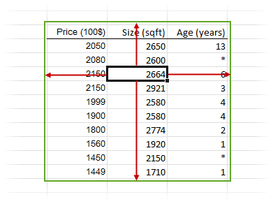
Most Excel commands (for example, Sort, Pivot Table) use the same technique to determine the range of cells to operate on. It avoids the need to select often-large ranges of cells using the mouse, which is laborious and error-prone. It also ensures that if you add, or remove, cases or variables, that subsequent analyses automatically reflect any changes to the dataset.
When you analyze data, any data in hidden rows on the worksheet are excluded. This feature lets you easily limit analysis to a subset of the cases in the dataset. You can hide rows manually or use a filter to hide them based on criteria.
You can locate a dataset anywhere on a worksheet, and you can keep multiple datasets on a single worksheet provided you separate them from each other by at least one blank row and column. However, we recommend that you use a separate worksheet for each dataset. Using separate worksheets allows you to name datasets using the Excel worksheet tabs, navigate between datasets using the worksheet tabs, and ensures that filtering a dataset does not affect other datasets on the same worksheet.
A variable is an attribute of an object. The value of a variable can vary from one thing to another.
Record quantitative data as the numeric value.
Record qualitative data as a numeric coding (for example, 0, 1, 2) or labels (for example, Low, Medium, High). Numeric codings are often preferred as they succinctly represent the values and allow quicker data entry. However, codings can be difficult to understand by anyone other than the person who assigned them. To make their meaning clear, you can also assign a label to each numeric coding.
Data are ordered based on numeric value, numeric coding, or if a numeric coding is not used into alphabetical label order. For some statistical tests, the sort order determines how observations are rank-ordered and can affect the results. Often alphabetic sort order does represent the correct ordering. For example Low, Medium, High is sorted alphabetically into High, Low, Medium which does not represent their correct, natural order. In such cases, you must explicitly set the order before analyzing the data.
Five different scales are used to classify measurements based on how much information each measurement conveys.
The different levels of measurement involve different properties of the numbers or symbols that constitute the measurements and also an associated set of permissible transformations.
| Measurement scale | Properties | Permissible transformation |
|---|---|---|
 Nominal Nominal |
Two things are assigned the same symbol if they have the same value of the attribute. For example, Gender (Male, Female); Religion (coded as 0=None, 1=Christian, 2=Buddhist). |
Permissible transformations are any one-to-one or many-to-one transformation, although a many-to-one transformation loses information. |
 Ordinal Ordinal |
Things are assigned numbers such that the order of the numbers reflects an order relation defined on the attribute. Two things x and y with attribute values a(x) and a(y) are assigned numbers m(x) and m(y) such that if m(x) > m(y), then a(x) > a(y). For example, Moh's scale for the hardness of minerals; academic performance grades (A, B, C, ...). |
Permissible transformations are any monotone increasing transformation, although a transformation that is not strictly increasing loses information. |
 Interval Interval |
Things are assigned numbers such that differences between the numbers reflect differences of the attribute. If m(x) - m(y) > m(u) - m(v), then a(x) - a(y) > a(u) - a(v). For example, Temperature measured in degrees Fahrenheit or Celsius. |
Permissible transformations are any affine transformation t(m) = c * m + d, where c and d are constants; another way of saying this is that the origin and unit of measurement are arbitrary. |
 Ratio Ratio |
Things are assigned numbers such that differences and ratios between the numbers reflect differences and ratios of the attribute. For example, Temperature measured in degrees Kelvin scale; Length in centimeters. |
Permissible transformations are any linear (similarity) transformation t(m) = c * m, where c is a constant; another way of saying this is that the unit of measurement is arbitrary. |
 Absolute Absolute |
Things are assigned numbers such that all properties of the numbers reflect analogous properties of the attribute. For example, Number of children in a family, Frequency of occurrence. |
The only permissible transformation is the identity transformation. |
While the measurement scale cannot determine a single best statistical method appropriate for data analysis, it does define which statistical methods are inappropriate. Where possible the use of a variable is restricted when its measurement scale is not appropriate for the analysis. For example, a nominal variable cannot be used in a t-test.
When the measurement scale of a variable is unknown, the scale is inferred from its role in the analysis and the type of data in the variable. If the measurement scale cannot be inferred, you must set the measurement scale.
Missing values occur when no data is recorded for an observation; you intended to make an observation but did not. Missing data are a common occurrence and can have a significant effect on the statistical analysis.
Missing values arise due to many reasons. For example, a subject dropped out of the study; a machine fault occurred that prevented a measurement been taken; a subject did not answer a question in a survey; or a researcher made a mistake recording an observation.
A missing value is indicated by an empty cell or a . (full stop) or * (asterisk) in the cell. These values always indicate a missing value, regardless of measurement scale of the variable. Similarly, cell values that are not valid for the measurement scale of the variable are treated as missing. For example, a cell containing text or a #N/A error value is treated as missing for a quantitative measurement scale variable, since neither are valid numeric values.
Some applications, especially older statistical software, use special values such as 99999 to indicate missing values. If you import such data, you should use the Excel Find & Replace command to replace the values with a recognized missing indicator.
In the presence of missing values you often still want to make statistical inferences. Some analyses support techniques such as deletion, imputation, and interpolation to allow the analysis to cope with missing values. However, it is still important before performing an analysis that you understand why the data is missing. When the reason for the missing data is not completely random, the study may be biased, and the statistics may be misleading.
Most data are available in case form with data for each sampling unit. Sometimes data are not available for each unit but are already summarized by counting the frequency of occurrences of each value, called frequency form data.
Whenever possible you should record data in case form. Case form data can be reduced to frequency form, but frequency form data cannot be reconstructed into case form. You may want to use frequency form data when working with a large amount of data from a database, where you can save computing resources by letting the database server tabulate the data.
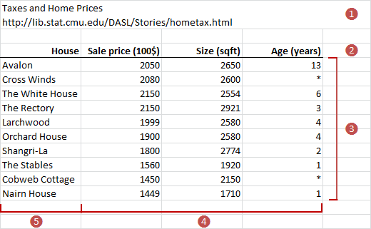
Each column is a variable (Height, Eye color), each row is a separate case (Subject) with the values of the variables on that case.
| Subject (optional) | Height | Eye color |
|---|---|---|
| 1 | 175 | Blue |
| 2 | 180 | Blue |
| 3 | 160 | Hazel |
| 4 | 190 | Green |
| 5 | 180 | Green |
| 6 | 150 | Brown |
| 7 | 140 | Blue |
| 8 | 160 | Brown |
| … | … | … |
Each column is a variable (Eye color) and a separate column for the number of cases (Frequency), each row is a combination of categories with the frequency count.
| Eye color | Frequency |
|---|---|
| Brown | 221 |
| Blue | 215 |
| Hazel | 93 |
| Green | 64 |
Set the measurement scale of a variable so data analysis can use the variable correctly.
Set the minimum/maximum and units so that the axes of charts are scaled to your preferences.
Set the order of categories for data analysis and output in the analysis report.
Set the precision of the data so that the results of the analysis show to a suitable number of decimal places.
Set a variable to use for labeling data points in plots for easy identification.
Assign labels to a numerical coding to make an analysis report more readable.
Assign colors or symbols to highlight observations on plots.
Transform a variable to normalize, shift, scale or otherwise change the shape of the distribution so that it meets the assumptions of a statistical test.
Useful Microsoft Excel functions for transforming data.
| Transform | Excel function |
|---|---|
| Natural log | =LN(cell) |
| Inverse natural log | =EXP(cell) |
| Reciprocal | =1 / cell |
| Square root | =SQRT(cell) |
| Power | =cell^power |
| Log base 10 | =LOG(cell) or =LOG10(cell) |
| Inverse log base 10 | =10^cell |
| Log base 2 | =LOG(cell, 2) |
| Inverse log base 2 | =2^cell |
Use an Excel filter to show only the rows that match a value or meet a condition. Rows that do not match the condition are hidden temporarily, and subsequent data analysis excludes them. This feature is extremely useful when you want to see how the analysis changes for a different subset of the data.
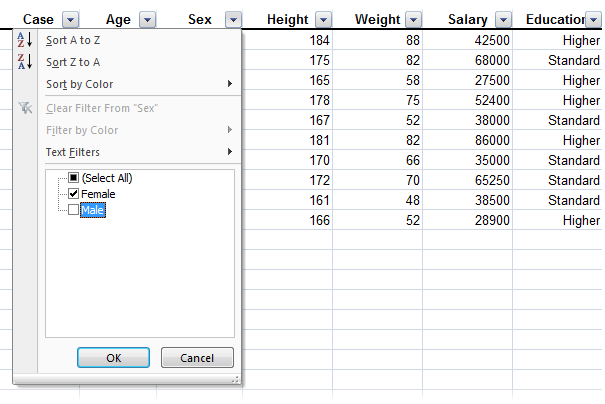
To filter to Female cases only, click the drop-down button alongside Sex, and then select Female in the list of values to match against:
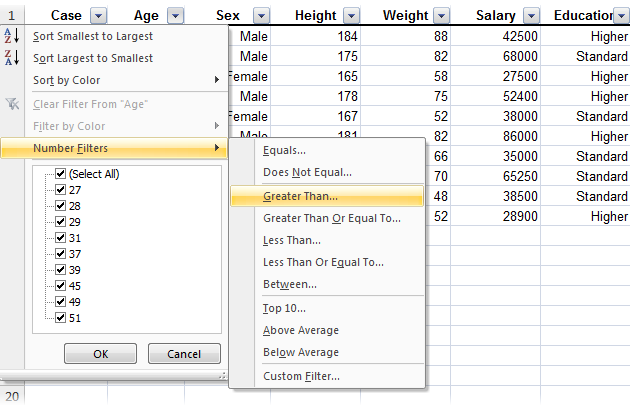
To filter to cases where the subject is older than 40, click the drop-down button alongside Age, and then click , and then enter 40 as the cut-off point: