The tools behind better diagnostic decisions Diagnostic accuracy with ROC curves and AUC comparison, Bland-Altman method agreement, reference intervals and survival analysis with Kaplan-Meier and Cox regression. The full general statistics toolkit for hypothesis testing, ANOVA and regression is included.

Every feature from all five editions for 15 days.
Medical edition from US$ 340 a year · 30-day money-back guarantee.
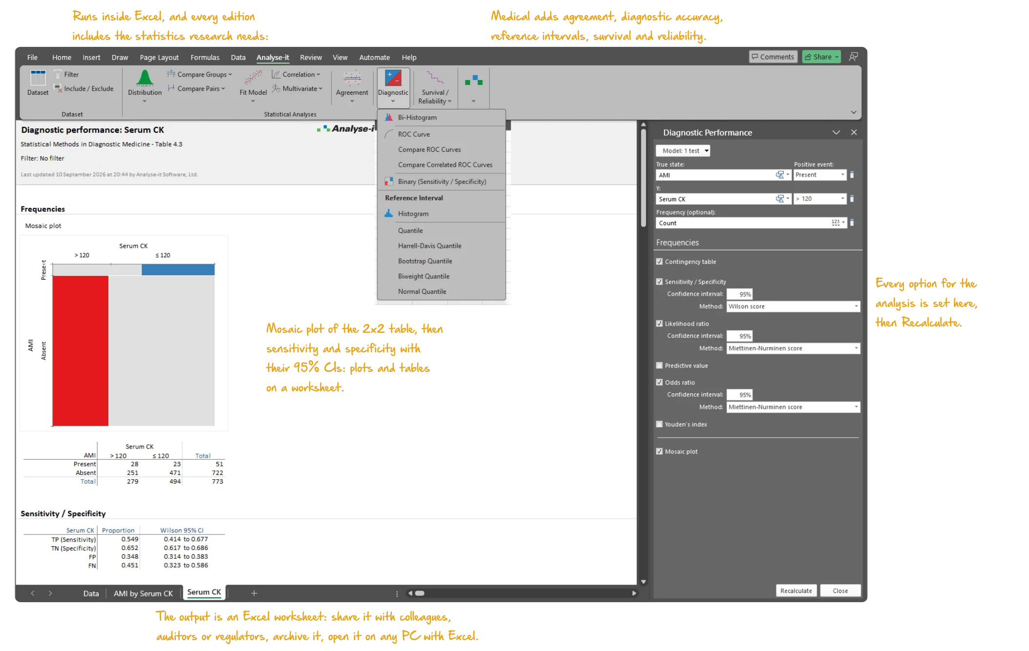
Microsoft Excel with the Analyse-it tab of the Medical edition selected: a diagnostic performance report for serum CK with the mosaic plot of the 2x2 table, the frequencies and the sensitivity and specificity table with confidence intervals, the Diagnostic Performance task pane open, and the Diagnostic menu dropped open on the ribbon listing the ROC, binary and reference interval commands. Handwritten notes: Runs inside Excel, and every edition includes the statistics research needs:; Medical adds agreement, diagnostic accuracy, reference intervals, survival and reliability; Mosaic plot of the 2x2 table, then sensitivity and specificity with their 95% CIs: plots and tables on a worksheet; Every option for the analysis is set here, then Recalculate; The output is an Excel worksheet: share it with colleagues, auditors or regulators, archive it, open it on any PC with Excel.

Clinical researchers, laboratory scientists and biostatisticians need specialised analyses that general-purpose statistics packages either do not include or bury in add-on modules.

The edition covers ROC curves for evaluating a diagnostic test, Bland-Altman for comparing measurement methods, reference intervals for establishing normal ranges and survival analysis for time-to-event data. The t-tests, ANOVA, regression and descriptive statistics that support every study sit alongside them.

The Medical edition brings all of this together in one package inside Excel. No separate applications for different analyses, no data export, no cloud processing. Analyse-it is cited in thousands of peer-reviewed publications.

Analyse-it has helped tremendously. Previously I used Prism and Microsoft Excel, but Analyse-it has made my life so much easier and saved so much time.
Man Khun Chan, M.Sc., ART
Test Development Medical Technologist
The Hospital For Sick Children, Toronto, Canada

Evaluate diagnostic test accuracy

Establish and compare the ability of a diagnostic test to discriminate between patients with and without a condition. Then find the decision threshold that balances sensitivity, specificity and clinical cost:

  • Empirical ROC curves, with the area under the curve, its DeLong confidence interval and the test against no discrimination
  • AUC comparison (DeLong) for up to 10 paired or independent tests — the difference in AUC with its confidence interval, and equality, equivalence or non-inferiority hypotheses
  • Sensitivity, specificity, likelihood ratios, predictive values at a prior probability, and the diagnostic odds ratio — each with its confidence interval
  • Optimal decision threshold by Youden’s index, the point closest to (0,1) or the clinical costs of misdiagnosis — and the sensitivity and specificity at any threshold
  • Decision plots of sensitivity and specificity, likelihood ratios, predictive values or cost across every possible threshold — where to set the cut-off, and what it costs
  • Qualitative test evaluation — sensitivity and specificity with confidence intervals, and the difference between two tests, for a test read as positive or negative against a known state
Diagnostic accuracy details →
Microsoft Excel showing the ROC Curve section of a diagnostic performance report: ROC curves for OxLDL and LDL, and the AUC table with DeLong 95% confidence intervals, SE, Z statistic and p-value for each test, with the task pane open on ROC Curve. Handwritten notes: ROC curve for each test; AUC with DeLong 95% CI, Z test and p-value; AUC estimator, CI and method.
ROC curves for OxLDL and LDL on one chart, and the AUC of each test with its DeLong 95% confidence interval, standard error, Z statistic and p-value.

Compare method agreement

When introducing a new analyser or comparing a point-of-care device against a laboratory method, see whether the two methods agree well enough for clinical use:

  • Bland-Altman limits of agreement with the bias as a mean, a median or a linear fit across the measuring range, each with a confidence interval on the limits
  • Constant and non-constant precision — regression-based, V-shaped limits of agreement when the differences grow with the concentration
  • Mountain plot — the folded CDF of the differences, with the allowable difference band, so the share of results within the allowance is read at once
  • Singlicate, duplicate and replicate measurements — with replicates the within-subject variance is estimated and the limits allow for it
  • Qualitative agreement between two tests — positive and negative percent agreement, kappa and weighted kappa — when the result is a category rather than a value
Bland-Altman agreement details →
Microsoft Excel showing a method comparison report for LDL cholesterol: the Bland-Altman difference plot with the 95% limits of agreement and the allowable difference band, with the task pane open on Fit Differences. Handwritten notes: Difference plot: Y - X against X; 95% limits of agreement and the allowable difference band; Bias model: mean, median or linear fit; limits.
LDL cholesterol, 100 samples, from EP21-A Table 2: the difference plot with the 95% limits of agreement and the ±10 mg/dL allowable difference band.

Establish reference intervals for clinical interpretation

The full range of reference interval methods lets you match the method to your sample size and distribution. Partition where subgroups need separate ranges, and screen for outliers before the limits are estimated:

  • Five quantile methods — parametric, non-parametric (three computation approaches), robust bi-weight, bootstrap and Harrell-Davis — the right estimator for the sample size and the shape of the data
  • Partition by sex, age, ethnicity or any combination of factors — one analysis per partition, with the descriptive statistics and limits for each
  • Full range of transformations — log, square root, cube root, Box-Cox, Manly exponential, two-stage exponential/modulus — for skewed analytes, with the limits reported back in the original units
  • Outlier screening with Tukey box plots, and Shapiro-Wilk and Anderson-Darling normality tests — the checks EP28-A3c asks for before the limits are estimated
Reference interval details →
Microsoft Excel showing a reference interval report for ALT in females: the raw histogram with its reference limits, and beneath it the Transformed histogram of ln ALT with a normal curve overlaid, with the task pane open on the Transform section. Handwritten notes: Raw ALT: skewed, with its reference limits; The same data after a log transform, normal curve overlaid; Transform: log, Box-Cox, Manly or two-stage modulus.
ALT in females: the raw histogram with its reference limits, and beneath it the same data after a natural log transformation with the normal curve overlaid.

Analyse time-to-event data with survival analysis

Estimate survival functions, compare treatment groups and model the effect of covariates on the hazard:

  • Kaplan-Meier survival curve for each group with pointwise, Nair or Hall-Wellner confidence bands, and the censored observations marked on the curve
  • Median, quartile and restricted mean survival time for each group, each with its confidence interval, and the survival function as a table
  • Test equality of the survival functions with the log-rank, Wilcoxon, Tarone-Ware or Fleming-Harrington test — the weighting chosen for early or late differences
  • Cox proportional hazards regression — the hazard ratio for every term with its confidence interval, interactions between factors and the baseline survival function
  • Log and log–log diagnostic plots for the proportional hazards assumption — curves that stay parallel support the model, curves that cross do not
Survival analysis details →
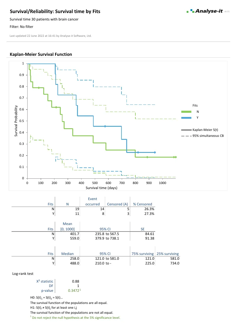
Microsoft Excel showing a survival analysis report: Kaplan-Meier survival curves for three tumour grades with censored observations marked, and the N, events, mean and median tables beneath, with the task pane open on the survival function options. Handwritten notes: A survival curve for each tumour grade; N, events, mean and median survival; Band: pointwise, Nair or Hall-Wellner.
Kaplan-Meier survival curves for 30 brain cancer patients grouped by tumour grade, censored observations marked on each curve.

Compare treatment groups and test for differences

The baseline demographics table, the primary endpoint comparison, the subgroup analysis — hypothesis testing is central to clinical research:

  • Student’s t, Welch’s t and Wilcoxon-Mann-Whitney for two independent groups; one-way ANOVA, Welch’s ANOVA and Kruskal-Wallis for three or more — with the homogeneity of variance tests that decide between them
  • Paired t-test, Wilcoxon signed ranks and Sign test for two related measurements; within-subjects ANOVA and Friedman for repeated measures on three or more occasions
  • Eight multiple comparison procedures — Tukey-Kramer, Dunnett, Hsu, Scheffé, Steel, Dwass-Steel-Critchlow-Fligner among them — to find which groups differ after a significant ANOVA, each controlling the family-wise error rate
  • Cohen’s d and Hedges’ g effect sizes with non-central t confidence intervals — how large the difference is, not only whether it is significant
  • Contingency tables — Pearson χ² and Fisher exact tests for independence, McNemar for related tables and the odds ratio and risk ratio with confidence intervals
Hypothesis testing details →
Microsoft Excel showing a Compare Pairs report for body fat before and after an exercise programme: side-by-side box plots with a line joining each of the 28 pairs, the descriptive statistics for Before, After and the differences beneath, and the Compare Pairs task pane open on Descriptives. Handwritten notes: Before and after for each subject, joined; box plots for each measure; Descriptives of the pairs and their differences; Connect the pairs.
Body fat before and after an exercise programme, 28 pairs: box plots with a line for each pair, and the descriptive statistics for Before, After and the differences.

Model risk factors and outcomes with regression

Simple and multiple linear regression, logistic regression with odds ratios, ANOVA and ANCOVA — with the diagnostics to know whether you can trust the result:

  • Simple, multiple, polynomial, logarithmic, exponential, power and probit regression — model a response on one predictor or many, with a confidence band on the fit
  • Binary logistic regression for a yes/no outcome — the odds ratio for every predictor with its Wald confidence interval, and likelihood ratio tests for the model and each term
  • ANOVA and ANCOVA with crossed factors, interactions and continuous covariates — effect means, main effect and interaction plots, and multiple comparisons on the effect means
  • Residual diagnostics, leverage plots, Cook’s D influence and VIF for multicollinearity — the checks that show whether a model can be trusted before it is reported
  • Predicted values for new observations from the fitted model
Regression details →
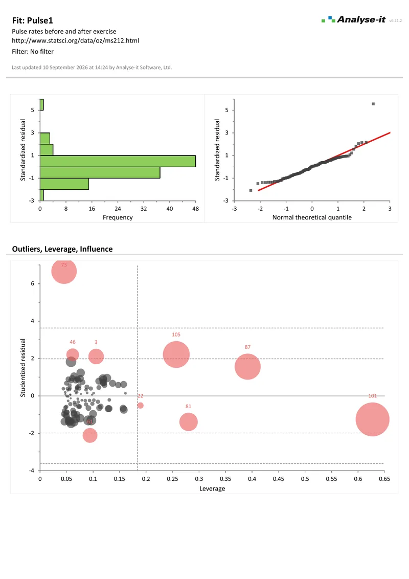
Microsoft Excel showing the Outliers, Leverage, Influence section of a multiple regression report of pulse rate on eight predictors: studentised residuals plotted against leverage for 109 observations, bubble size Cook's D, with the unusual cases labelled by observation number, and the Fit Model task pane open on the Outliers section. Handwritten notes: Studentised residual against leverage, bubble size Cook's D; influential cases labelled; Plot type, and labelling of influential cases.
Studentised residual against leverage for the 109 pulse-rate observations, bubble size Cook’s D, with the unusual cases labelled by observation number.

Describe and summarise your data

Every analysis starts with understanding the distribution:

  • Mean, median, SD, CV%, skewness, kurtosis, geometric mean and quantiles — the location and dispersion of a variable, with confidence intervals, in one table
  • Histograms, box plots, dot plots, CDF plots and Q-Q plots with Lilliefors bands — see the shape of the distribution, and any outliers, before choosing a test
  • Shapiro-Wilk, Anderson-Darling and Kolmogorov-Smirnov normality tests — a formal check on the assumption behind a t-test or ANOVA, alongside the Q-Q plot
  • One-sample t-test, Wilcoxon and Sign test for location, and the χ² test for variance. Test a mean, median or SD against a hypothesised value, with the confidence interval alongside
  • Correlation — Pearson r, Spearman rs and Kendall τ for every pair of variables, each with a confidence interval and test. A scatter plot matrix shows the relationships
  • PCA and common factor analysis — reduce many correlated variables to a few components or factors, with biplots and 12 orthogonal and oblique rotation methods
Descriptive statistics details →
Microsoft Excel showing the Frequencies section of a discrete distribution report for the eye colour of 592 people: the bar plot of relative frequency for brown, blue, hazel and green, the pie plot beneath it, the frequency table, and the Distribution task pane open. Handwritten notes: Frequency bar chart with the cumulative relative frequency line; Whole-to-part pie chart, sectors labelled; Plot: bar or pie, with the cumulative line.
Eye colour of 592 people: the bar plot of relative frequency and the pie plot from the discrete distribution analysis, with the task pane open.
Analyse-it has a tremendous advantage in its ease of use. With other programs, you really have to study how to use them, but Analyse-it makes it so easy, and at the same time offers the advanced procedures we need.
Marco Balerna, Ph.D.
Clinical Chemist
Ente Ospedaliero Cantonale, Switzerland
Read the case study →

Includes the full Standard edition

The Medical edition includes every feature from the Standard edition — the general-purpose statistics toolkit that clinical researchers use for the rest of the study. Baseline demographics, treatment group comparisons, outcome modelling and exploratory analysis are all in the same workbook as your Bland-Altman, ROC and survival analyses.

Related guides in the Learn section: ROC curves and AUC explained, Bland-Altman limits of agreement, choosing a reference interval method and Kaplan-Meier survival curves.


Software you can trust

Validated calculations you can defend at peer review Every calculation is performed by Analyse-it — no Excel formulas, no third-party functions. Results are validated against published datasets and thousands of internal test cases before every release. How Analyse-it is developed and validated →
Patient data stays on your PC Analyse-it runs entirely within Microsoft Excel on your PC. No cloud processing, no data transmission. Patient data and research data stay within your facility under your own data governance controls.
Standard Excel workbooks anyone can open Every analysis is an ordinary .xlsx workbook. Share with co-authors, attach to a manuscript submission, archive for publication queries. No proprietary format, no licence required to view results. Co-authors and reviewers see exactly what you see.
Results that cannot be accidentally broken Analysis output contains computed values, not formulas. Nothing to accidentally overwrite, no cell references to break, no formula errors to introduce. The results you published are exactly what you will find when you reopen the workbook months or years later, when a reviewer asks.

Example analyses

Download example datasets, open them in the trial and see exactly what the output looks like.

EP24 A2 Example 1 2 pages EP24-A2 — Appendix D
OxLDL and LDL diagnostic accuracy.
50 subjects, 28 of them with the condition. ROC curves for both markers with AUC, CIs and a test against 0.5 — OxLDL 0.80, LDL 0.56 — and a DeLong comparison of the two curves. A second analysis adds the bi-histogram and decision threshold plot for OxLDL alone.
EP21 A Example 1 2 pages EP21-A — Table 2
LDL cholesterol total analytical error.
100 observations. Difference plot and mountain plot with an allowable difference of ±10 mg/dL, median difference with a 90% CI and 95% limits of agreement.
EP28 A3 Example 1 2 pages EP28-A3c — Table 4
Calcium reference intervals by sex.
120 observations per sex, reported separately. Distribution with descriptive statistics, and nonparametric reference limits from the (N+1)p quantile with 90% CIs.
Kaplan Meier 3 pages Kaplan-Meier survival
Brain cancer survival, 30 patients.
Two analyses of one dataset — survival by treatment, 19 patients against 11 and survival by tumour grade over three groups. Survival curves with confidence bands, mean and median survival with CIs, quartile survival times and a log-rank test for each.
EP12 A2 Example 1 2 pages EP12-A2 — Example 10.3.1
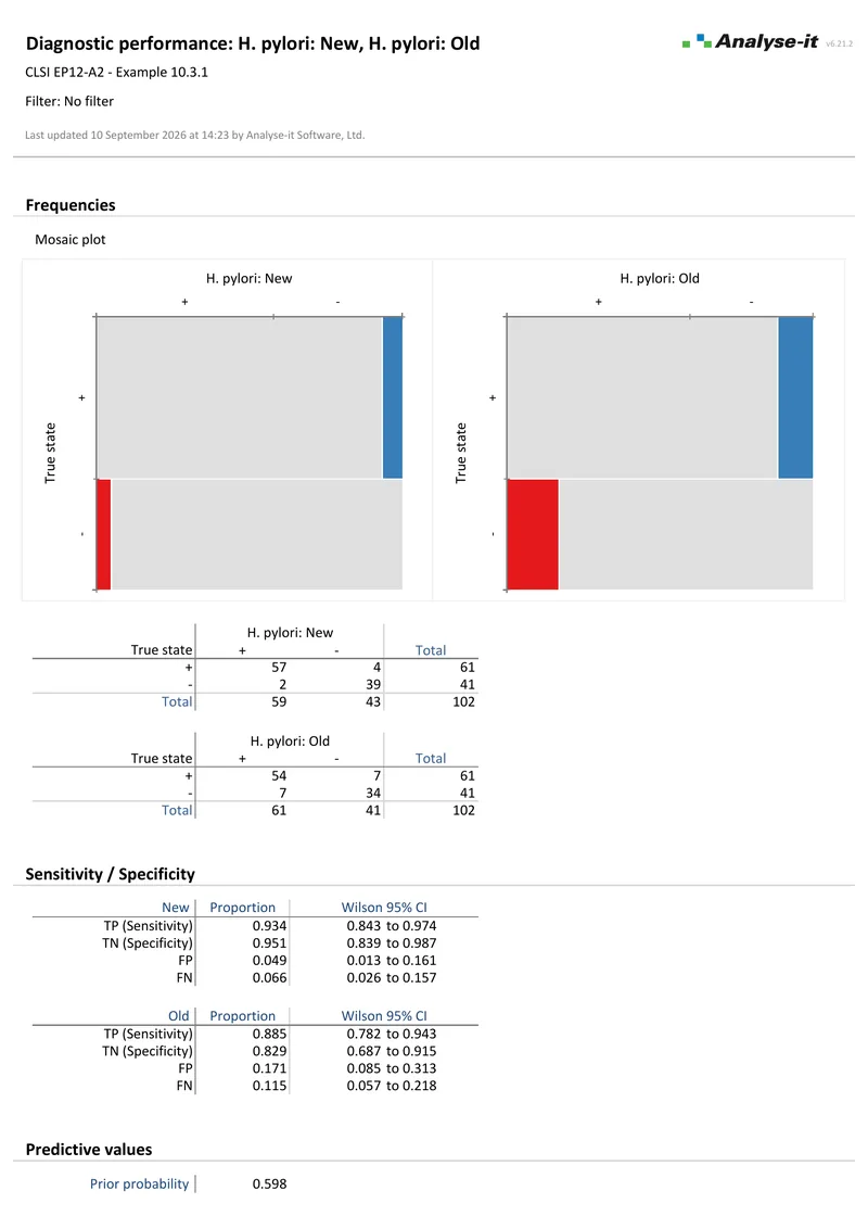
H. pylori, two qualitative tests against a known state.
102 subjects. Mosaic plots, sensitivity and specificity with Wilson 95% CIs and predictive values at the observed prior. The difference between the two tests with Newcombe CIs and a score Z test.
Compare Groups 1 3 pages One-way ANOVA
Y by brand, 7 groups, 19 observations.
Descriptive statistics by group, Levene test for homogeneity of variance, one-way ANOVA, Tukey-Kramer all-pairs comparisons over 21 contrasts with simultaneous 95% CIs and a Mean-Mean scatter plot.
Fit Model 2 p4 4 pages Multiple regression
Pulse rates before and after exercise, 8 predictors.
109 observations, three continuous predictors and five categorical. Parameter estimates with 95% CIs and VIF, F tests for each term, leverage plots for every predictor, residual diagnostics and an outlier, leverage and influence plot.
Fit Model 3 2 pages Binary logistic regression
Intensive care unit survival, 17 predictors.
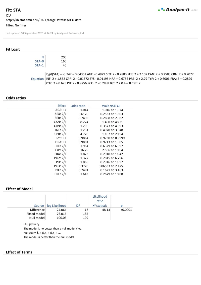
200 observations. Odds ratios with Wald 95% CIs and likelihood ratio tests for the model and for each term. Age, cancer, CPR, systolic blood pressure and admission type are significant at 5%.

Free trial and pricing

Try it on your own data first. The 15-day trial is every feature from all five editions — install it and start straight away.

Medical edition: US$ 340 per year or US$ 815 for a perpetual licence. Every purchase carries a 30-day money-back guarantee. Need a quote for purchasing? Add the licence to the cart and save it as a PDF quote.

Technical details

Diagnostic accuracy

ROC analysis

  • 1 test, up to 10 paired tests or up to 10 independent tests/groups
  • Empirical (non-parametric) ROC curves
  • ROC curve plot with the no-discrimination line
  • Overlaid ROC curves for test comparison
  • Wilcoxon-Mann-Whitney AUC with DeLong-DeLong-Clarke-Pearson CI
  • Z test that the AUC exceeds 0.5 (no discrimination)
  • Compare DeLong AUC difference — equality, equivalence or non-inferiority
  • Comparisons for all pairs of tests or each against a control
  • Number of TP, TN, FP, FN
  • Sensitivity, specificity with Clopper-Pearson exact or Wilson score CI
  • Positive and negative likelihood ratios
  • Positive and negative predictive values
  • Predictive values at multiple prior probabilities (prevalences) new in v5.51
  • Diagnostic odds ratio and Youden index
  • Optimal threshold: Youden, closest-to-(0,1), cost-based
  • Decision plot: sensitivity/specificity, likelihood ratios, predictive values or cost vs threshold
  • Bi-histogram and dot plot
  • Predict FPF at fixed sensitivity, sensitivity at fixed FPF or sensitivity/FPF at fixed threshold

Qualitative test evaluation

  • 1 test, 2 paired tests or 2 independent tests/groups
  • Sensitivity, specificity with Clopper-Pearson exact or Wilson score CI
  • Positive and negative likelihood ratios with Miettinen-Nurminen score CI
  • Predictive values at the observed or a specified prevalence, with Mercaldo-Wald logit CI
  • Diagnostic odds ratio and Youden index
  • Mosaic plot of outcomes
  • Difference between sensitivity/specificity with Newcombe score CI, plus Tango score CI for paired tests and Miettinen-Nurminen score CI for independent tests
  • Equivalence and non-inferiority tests for sensitivity/specificity new in v5.65
  • McNemar-Mosteller exact, Fisher exact and score Z test

Agreement (Bland-Altman)

Quantitative methods

  • Singlicate, duplicate and replicate measurements
  • Bland-Altman limits of agreement with mean, median and linear fit bias
  • Limits of agreement — constant and non-constant precision
  • Confidence intervals on limits of agreement
  • Non-parametric (percentile) limits of agreement
  • Limits of agreement for single measurements or for the mean of replicates
  • Allowable difference specification and overlay
  • Within-subject variance estimation from replicates
  • Precision (SD or CV) for each method
  • Pearson r correlation coefficient

Qualitative methods

  • Proportion in positive/negative agreement with Clopper-Pearson exact or Wilson score CI
  • Kappa and weighted kappa (linear or quadratic weights) with Wald Z CI
  • Kappa test for agreement
  • Bangdiwala agreement plot new in v5.60
  • Dice-Sørensen average agreement new in v5.60

Plots

  • Scatter plot with identity line
  • Difference / relative difference / ratio plot with allowable difference band and histogram
  • Mountain plot with allowable difference band
  • Vary colour of points by a factor
  • Linear or log X-axis on difference plots new in v5.51

Reference intervals

Establish reference limits

  • Normal (parametric) quantile, Z (MVUE) or t-based
  • Non-parametric quantile: (N+1)p, Np+½, (N+⅓)p+⅓
  • Harrell-Davis quantile
  • Bootstrap quantile
  • Robust bi-weight quantile
  • Confidence intervals on all reference limits
  • Bootstrap confidence intervals
  • Two-sided reference interval or one-sided reference limit

Partitioning & transformations

  • Partition by factor(s)
  • Reciprocal, log, square and cube root
  • Box-Cox
  • Manly exponential
  • Two-stage exponential / modulus

Normality & outliers

  • Shapiro-Wilk test
  • Anderson-Darling test
  • Normal Q-Q plot with Lilliefors confidence band
  • Frequency histogram with normal overlay and reference limits
  • Tukey outlier box plot

Survival / reliability

Survival function new in v6.10

  • Kaplan-Meier survival curve with pointwise, Nair or Hall-Wellner confidence bands
  • Median and quartiles for survival/failure
  • Mean (area under survival curve) and restricted mean
  • Survival/failure probabilities and confidence intervals
  • Full or abbreviated survival function table with censored observations marked
  • Test equality: log-rank, Wilcoxon, Tarone-Ware, Fleming-Harrington
  • Transformed log and log–log S(t) vs time plots

Cox proportional hazards new in v6.01

  • Model equation
  • Parameter estimates and Wald confidence intervals
  • Covariance of estimates
  • Baseline survival function and plot
  • Likelihood ratio and Wald test of model and terms
  • Hazard ratio at each level / specified unit change and at specific levels of interacting covariates

Included from the Standard edition

The Medical edition includes every feature from the Standard edition. See the Standard edition page for the full technical specification, including:

  • Descriptive statistics, histograms, box plots, dot plots, Q-Q plots, normality tests
  • Compare groups: t-test, Welch, Wilcoxon, ANOVA, Kruskal-Wallis, 8 multiple comparison procedures
  • Compare pairs: paired t-test, Wilcoxon signed ranks, Friedman, within-subject ANOVA
  • Effect sizes: Cohen’s d, Hedges’ g, Hodges-Lehmann
  • Contingency tables: Pearson χ², Fisher exact, McNemar, odds/risk ratios
  • Simple, multiple and polynomial regression with diagnostics; logistic regression
  • ANOVA/ANCOVA with effect means, interaction plots, multiple comparisons
  • Correlation: Pearson r, Spearman rs, Kendall τ
  • PCA, common factor analysis, biplots, 12 rotation methods
  • Cronbach’s alpha

System requirements

  • Excel 365, 2024, 2021, 2019 or 2016 for Windows (32- and 64-bit)
  • Windows 11 or 10, or Windows Server 2016 onwards
  • 2 GB RAM minimum recommended
  • 80 MB disk space