
A discrete distribution describes a variable that can only take discrete values (for example, the number of male and females, or the number of people with a specific eye color).
A frequency distribution reduces a large amount of data into a more easily understandable form.
A frequency table is a simple table of the frequencies in each class.
| Statistic | Purpose |
|---|---|
| Frequency | The number of occurrences in the class. |
| Relative frequency | The frequency divided by the total. |
| Frequency density | The relative frequency divided by the width of the class interval. Use with unequal class intervals. |
| Cumulative frequency | The number of occurrences in the class and all previous classes. |
| Cumulative relative frequency | The cumulative frequency divided by the total. |
A frequency plot shows the distribution of a qualitative variable.
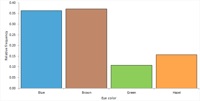
A frequency plot shows rectangular bars for each class with the height of the bar proportional to the frequency.
A whole-to-part plot shows how the parts make up the whole.

A pie chart is a common representation which shows a circle divided into sectors for each class, with the angle of each sector proportional to the frequency.
A stacked bar plot shows rectangular bars for each class with the size of each bar proportional to the frequency.
The major problem with the pie chart is that it is difficult to judge the angles and areas of the sectors. It is useful if you want to compare a single class relative to the whole. For comparing classes to each other, we recommend the frequency plot or stacked bar plot for greater clarity and ease of interpretation.
Plot a frequency plot to visualize the distribution of a qualitative variable.
Plot a pie chart or bar chart to visualize the relative frequencies.
Inferences about the parameters of a binomial distribution are made using a random sample of data drawn from the population of interest.
A binomial distribution arises when an experiment consists of a fixed number of repeated trials; each trial has two possible outcomes; the probability of the outcome is the same for each trial; and the trials are independent, that is, the outcome of one trial does not affect the outcome of other trials.
A parameter estimate is either a point or interval estimate of an unknown population parameter.
A point estimate is a single value that is the best estimate of the true unknown parameter; a confidence interval is a range of values and indicates the uncertainty of the estimate.
Estimators for the binomial distribution parameter and their properties and assumptions.
| Estimator | Purpose |
|---|---|
| Proportion | Estimate the population proportion of occurrences of the outcome of interest using the sample proportion estimator. |
| Odds | Estimate the population odds of the outcome of interest occurring using the sample odds estimator. Odds is an expression of the relative probabilities in favor of an event. |
A hypothesis test formally tests if a population parameter is equal to a hypothesized value. For a binomial distribution, the parameter is the probability of success, commonly referred to as the proportion with the outcome of interest.
The null hypothesis states that the proportion is equal to the hypothesized value, against the alternative hypothesis that it is not equal to (or less than, or greater than) the hypothesized value. When the test p-value is small, you can reject the null hypothesis and conclude the sample is not from a population with the proportion equal to the hypothesized value.
Tests for the parameter of a binomial distribution and their properties and assumptions.
| Test | Purpose |
|---|---|
| Binomial exact | Test if the proportion with the outcome of interest is equal to a hypothesized value. Uses the binomial distribution and computes an exact p-value. The test is conservative, that is, the type I error is guaranteed to be less than or equal to the desired significance level. Recommended for small sample sizes. |
| Score Z | Test if the proportion with the outcome of interest is equal to a hypothesized value. Uses the score statistic and computes an asymptotic p-value. Equivalent to Pearson's X² test. Recommended for general use. |
Test if the parameter of a binomial distribution is equal to the hypothesized value.
Inferences about the parameters of a multinomial distribution are made using a random sample of data drawn from the population of interest.
A multinomial distribution arises when an experiment consists of a fixed number of repeated trials; each trial has a discrete number of possible outcomes; the probability that a particular outcome occurs is the same for each trial; and the trials are independent, that is, the outcome of one trial does not affect the outcome of other trials.
A hypothesis test formally tests if the population parameters are different from the hypothesized values. For a multinomial distribution, the parameters are the proportions of occurrence of each outcome.
The null hypothesis states that the proportions equal the hypothesized values, against the alternative hypothesis that at least one of the proportions is not equal to its hypothesized value. When the test p-value is small, you can reject the null hypothesis and conclude that at least one proportion is not equal to its hypothesized value.
The test is an omnibus test and does not tell you which proportions differ from the hypothesized values.
Tests for the parameters of a multinomial distribution and their properties and assumptions.
| Test | Purpose |
|---|---|
| Pearson X² | Tests if the proportions are equal to the hypothesized values. Uses the score statistic and computes an asymptotic p-value. |
| Likelihood ratio G² | Tests if the proportions are equal to the hypothesized values. Uses the likelihood ratio statistic and computes an asymptotic p-value. Pearson X² usually converges to the chi-squared distribution more quickly than G². The likelihood ratio test is commonly used in statistical modeling as the G² statistic is easier to compare between different models. |
Test if the parameters of a multinomial distribution are equal to the hypothesized values.
Distribution analysis study requirements and dataset layout.
Use a column for each variable (Height, Eye color); each row has the values of the variables for a case (Subject).
| Subject (optional) | Height | Eye color |
|---|---|---|
| 1 | 175 | Blue |
| 2 | 180 | Blue |
| 3 | 160 | Hazel |
| 4 | 190 | Green |
| 5 | 180 | Green |
| 6 | 150 | Brown |
| 7 | 140 | Blue |
| 8 | 160 | Brown |
| 9 | 165 | Green |
| 10 | 180 | Hazel |
| … | … | … |
Use a column for the variable (Eye color) and a column for the number of cases (Frequency); each row has the values of the variables and the frequency count.
| Eye color | Frequency |
|---|---|
| Brown | 221 |
| Blue | 215 |
| Hazel | 93 |
| Green | 64 |


