Diagnostic performance

Diagnostic performance evaluates the ability of a qualitative or quantitative test to discriminate between two subclasses of subjects.

• Measures of diagnostic accuracy
  Diagnostic accuracy measures the ability of a test to detect a condition when it is present and detect the absence of a condition when it is absent.
• ROC plot
  ROC (receiver operating characteristic) curves show the ability of a quantitative diagnostic test to classify subjects correctly as the decision threshold is varied.
• Area under the curve (AUC)
  The area under (a ROC) curve is a measure of the accuracy of a quantitative diagnostic test.
• Difference between the areas under two curves
  The difference between areas under the ROC curves compares the accuracy of two or more diagnostic tests.
• Decision thresholds
  A decision threshold is a value that dichotomizes the result of a quantitative test to a simple binary decision.
• Decision plot
  A decision plot shows a measure of performance (such as sensitivity, specificity, likelihood ratios, or predictive values) against all decision thresholds to help identify optimal decision threshold.

Diagnostic accuracy measures the ability of a test to detect a condition when it is present and detect the absence of a condition when it is absent.

A perfect diagnostic test can discriminate all subjects with and without the condition and results in no false positive or false negatives. However, this is rarely achievable, as misdiagnosis of some subjects is inevitable. Measures of diagnostic accuracy quantify the discriminative ability of a test.

• Sensitivity / Specificity
  Sensitivity and specificity are the probability of a correct test result in subjects with and without a condition, respectively.
• Likelihood ratios
  Likelihood ratios are the ratio of the probability of a specific test result for subjects with the condition against the probability of the same test result for subjects without the condition.
• Predictive values
  Predictive values are the probability of correctly identifying a subject's condition given the test result.
• Youden J
  Youden's J is the likelihood of a positive test result in subjects with the condition versus those without the condition. It is also the probability of an informed decision (as opposed to a random guess).

Sensitivity and specificity are the probability of a correct test result in subjects with and without a condition, respectively.

Sensitivity (true positive fraction, TPF) measures the ability of a test to detect the condition when it is present. It is the probability that the test result is positive when the condition is present.

Specificity (true negative fraction, TNF) measures the ability of a test to detect the absence of the condition when it is not present. It is the probability that the test result is negative when the condition is absent.

Likelihood ratios are the ratio of the probability of a specific test result for subjects with the condition against the probability of the same test result for subjects without the condition.

A likelihood ratio of 1 indicates that the test result is equally likely in subjects with and without the condition. A ratio > 1 indicates that the test result is more likely in subjects with the condition than without the condition, and conversely, a ratio < 1 indicates that the test result is more likely in subjects without the condition. The larger the ratio, the more likely the test result is in subjects with the condition than without; likewise, the smaller the ratio, the more likely the test result is in subjects without than with the condition.

The likelihood ratio of a positive test result is the ratio of the probability of a positive test result in a subject with the condition (true positive fraction) against the probability of a positive test result in a subject without the condition (false positive fraction). The likelihood ratio of a negative test result is the ratio of the probability of a negative test result in a subject with the condition (false negative fraction) to the probability of a negative test result in a subject without the condition (true negative fraction).

Predictive values are the probability of correctly identifying a subject's condition given the test result.

Predictive values use Bayes' theorem along with a pre-test prior probability (such as the prevalence of the condition in the population) and the sensitivity and specificity of the test to compute the post-test probability (predictive value).

The positive predictive value is the probability that a subject has the condition given a positive test result; the negative predictive value is the probability that a subject does not have the condition given a negative test result.

Youden's J is the likelihood of a positive test result in subjects with the condition versus those without the condition. It is also the probability of an informed decision (as opposed to a random guess).

Youden's J index combines sensitivity and specificity into a single measure (Sensitivity + Specificity - 1) and has a value between 0 and 1. In a perfect test, Youden's index equals 1. It is also equivalent to the vertical distance above the diagonal no discrimination (chance) line to the ROC curve for a single decision threshold.

Estimate the sensitivity/specificity and other measures of the accuracy of a binary diagnostic test (or a quantitative test at a specific decision threshold).

1. Select a cell in the dataset.
2. On the Analyse-it ribbon tab, in the Statistical Analyses group, click Diagnostic, and then click Binary (Sensitivity / Specificity).
   The analysis task pane opens.
3. In the True state drop-down list, select the true condition variable.
4. In the Positive event drop-down list, select the state that indicates the presence of the condition/event of interest.
5. In the Y drop-down list(s), select the test variable(s).
6. If the Y variable is binary, in the Positive event drop-down list, select the state that indicates a positive test.
7. If the Y variable is quantitative, click the menu next to the variable and select Cut-off, and then enter the criteria to recode the variable into a binary variable.
8. If the data are in frequency form, in the Frequency drop-down list, select the frequency count variable.
9. Optional: Select the appropriate TP/TN/FP/FN, Sensitivity / Specificity, Likelihood ratio, Predictive value check boxes.
10. Click Calculate.

Compare the sensitivity and specificity of two diagnostic tests and make inferences about the differences.

1. Select a cell in the dataset.
2. On the Analyse-it ribbon tab, in the Statistical Analyses group, click Diagnostic, and then click Binary (Sensitivity / Specificity).
   The analysis task pane opens.
3. In the Model drop-down menu, select the number of tests and the type of study design.

   Option	Description
   2 paired tests	Compare 2 tests where the results are on the same subjects.
   2 independent tests / groups	Compare 2 tests where the results are on different subjects, or 1 test applied to 2 different groups of subjects.

4. In the True state drop-down list, select the true condition variable.
5. In the Positive event drop-down list, select the state that indicates the presence of the condition/event of interest.
6. If comparing 2 independent tests, in the Y drop-down list, select the diagnostic test variable, and then in the Factor drop-down list, select the factor variable (test or group indicator).
7. If comparing 2 paired tests, in the Y drop-down lists, select the diagnostic test variables.
8. If the data are in frequency form, in the Frequency drop-down list, select the frequency count variable.
9. On the Analyse-it ribbon tab, in the Diagnostic Accuracy group, click Test, and then click:

   Option	Description
   Equality	Test if the sensitivities/specificities of two tests are equal.
   Equivalence	Test if the sensitivities/specificities of two tests are equivalent within a practical difference.
   Non-inferiority	Test if the sensitivity/specificity of a new test is not inferior to a standard test.

   The default options use a Miettinen-Nurminen or Tango score confidence interval, and a Score Z test. The Newcombe score confidence interval is approximate not based on the same evidence function, and rejection of a hypothesis based on the confidence limits and hypothesis test may give conflicting results.

10. In the analysis task pane, under the hypotheses drop-down list:
    • If testing a hypothesis of equivalence, in the Equivalent difference, type the smallest practical difference that would be considered the same.
    • If testing a hypothesis of non-inferiority, in the Standard drop-down list, select the standard diagnostic test, and then in the Smallest difference edit box, type the smallest difference that would be considered inferior.
11. Optional: To compare the p-value against a predefined significance level, in the Significance level edit box, type the maximum probability of rejecting the null hypothesis when in fact it is true (typically 5% or 1%).
12. Click Calculate.

ROC (receiver operating characteristic) curves show the ability of a quantitative diagnostic test to classify subjects correctly as the decision threshold is varied.

The ROC plot shows sensitivity (true positive fraction) on the horizontal axis against 1-specificity (false positive fraction) on the vertical axis over all possible decision thresholds.

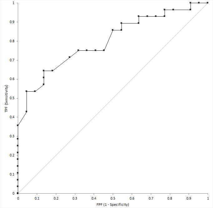
A diagnostic test able to perfectly identify subjects with and without the condition produces a curve that passes through the upper left corner (0, 1) of the plot. A diagnostic test with no ability to discriminate better than chance produces a diagonal line from the origin (0, 0) to the top right corner (1, 1) of the plot. Most tests lie somewhere between these extremes. If a curve lies below the diagonal line (0, 0 to 1, 1), you can invert it by swapping the decision criteria to produce a curve above the line.

An empirical ROC curve is the simplest to construct. Sensitivity and specificity use the empirical distributions for the subjects with and without the condition. This method is nonparametric because no parameters are needed to model the behavior of the curve, and it makes no assumptions about the underlying distribution of the two groups of subjects.

Plot the receiver-operator characteristic (ROC) curve to visualize the accuracy of a diagnostic test.

1. Select a cell in the dataset.
2. On the Analyse-it ribbon tab, in the Statistical Analyses group, click Diagnostic, and then under the Accuracy heading, click ROC Curve.
   The analysis task pane opens.
3. In the True state drop-down list, select the true condition variable.
4. In the Positive event drop-down list, select the state that indicates the presence of the condition/event of interest.
5. In the Y drop-down list, select the diagnostic test variable.
6. Optional: To show a bi-histogram of the distributions of the diagnostic test by the true condition, On the Analyse-it ribbon tab, in the Diagnostic Accuracy group, click Bi-Histogram
7. Optional: To show the diagnostic accuracy for each decision threshold, On the Analyse-it ribbon tab, in the Diagnostic Accuracy group, click Sensitivity / Specificity, Likelihood ratio, Predictive value.
8. Click Calculate.

Plot multiple receiver-operator characteristics (ROC) curves to make comparisons between them.

1. Select a cell in the dataset.
2. On the Analyse-it ribbon tab, in the Statistical Analyses group, click Diagnostic, and then under the Accuracy heading, click:

   Option	Description
   Compare ROC Curves	Compare 2 or more independent ROC curves.
   Compare Correlated ROC Curves	Compare 2 or more paired/correlated ROC curves.

   The analysis task pane opens.
3. In the True state drop-down list, select the true condition variable.
4. In the Positive event drop-down list, select the state that indicates the presence of the condition/event of interest.
5. If comparing 2 or more independent ROC curves, in the Y drop-down list, select the diagnostic test variable, and then in the Factor drop-down list, select the grouping variable.
6. If comparing 2 or more paired/correlated ROC curves, in the Y list, select the diagnostic test variables.
7. Click Calculate.

The area under (a ROC) curve is a measure of the accuracy of a quantitative diagnostic test.

A point estimate of the AUC of the empirical ROC curve is the Mann-Whitney U estimator (DeLong et. al., 1988). The confidence interval for AUC indicates the uncertainty of the estimate and uses the Wald Z large sample normal approximation (DeLong et al., 1998). A test with no better accuracy than chance has an AUC of 0.5, a test with perfect accuracy has an AUC of 1.

AUC can be misleading as it gives equal weight to the full range of sensitivity and specificity values even though a limited range, or specific threshold, may be of practical interest.

Test if the area under the curve is better than chance, or some other value.

1. Activate the analysis report worksheet.
2. On the Analyse-it ribbon tab, in the Diagnostic Accuracy group, click Test, and then click No Discrimination.

   The default null hypothesis is that the AUC is less than or equal to 0.5 against the alternative hypothesis that the AUC is greater than the 0.5. This tests if the AUC is better than chance alone.

   The analysis task pane ROC Curve panel opens.
3. Optional: In the Hypotheses drop-down list, select the null and alternative hypothesis.
4. Optional: In the Hypothesized value edit box, type the expected value of the parameter under the null hypothesis.
5. Optional: To compare the p-value against a predefined significance level, in the Significance level edit box, type the maximum probability of rejecting the null hypothesis when in fact it is true (typically 5% or 1%).
6. Click Recalculate.

The difference between areas under the ROC curves compares the accuracy of two or more diagnostic tests.

It is imperative when comparing tests that you choose the correct type of analysis dependent on how you collect the data. If the tests are performed on the same subjects (paired design), the test results are usually correlated. Less commonly, you may perform the different tests on different groups of subjects or the same test on different groups of subjects, and the test results are independent. A paired design is more efficient and is preferred whenever possible.

A point estimate of the difference between the area under two curves is a single value that is the best estimate of the true unknown parameter; a confidence interval indicates the uncertainty of the estimate. If the tests are independent, the confidence interval uses the combined variance of the curves and a large sample Wald approximation. If the tests are paired, the standard error incorporates the covariance (DeLong et al., 1998) and uses a large sample Wald approximation.

When the ROC curves cross, the difference between the AUC does not provide much useful information.

Test if the area under curves is equal, equivalent, or not inferior to another.

1. Activate the analysis report worksheet.
2. On the Analyse-it ribbon tab, in the Diagnostic Accuracy group, click Test, and then click:

   Option	Description
   Equality	Test if the AUCs are equal.
   Equivalence	Test if the AUCs are equivalent within a practical difference.
   Non-inferiority	Test if the AUC is not inferior to another AUC.

   The analysis task pane Comparisons panel opens.
3. In the analysis task pane, under the hypotheses drop-down list:
   • If testing a hypothesis of equivalence, in the Contrast drop-down list, select the comparisons, and then in the Equivalent difference, type the smallest practical difference that would be considered the same.
   • If testing a hypothesis of non-inferiority, in the Standard drop-down list, select the standard diagnostic test, and then in the Smallest difference edit box, type the smallest difference that would be considered inferior.
4. Optional: To compare the p-value against a predefined significance level, in the Significance level edit box, type the maximum probability of rejecting the null hypothesis when in fact it is true (typically 5% or 1%).
5. Click Recalculate.

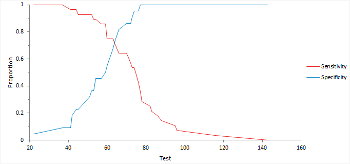
A decision threshold is a value that dichotomizes the result of a quantitative test to a simple binary decision.

The test result of a quantitative diagnostic test is dichotomized by treating the values above or equal to a threshold as positive, and those below as negative, or vice-versa.

There are many ways to choose a decision threshold for a diagnostic test. For a simple screening test, the decision threshold is often chosen to incur a fixed, true positive, or false positive rate. In more complex cases, the optimal decision threshold depends on both the cost of performing the test and the cost of the consequences of the test result. The costs may include both financial and health-related costs. A simple formula to determine the optimal decision threshold (Zweig & Campbell, 1993) maximizes: Sensitivity - m * (1- Specificity) where m = (Cost FP - Cost TN) / (Cost FN - Cost TP).

A decision plot shows a measure of performance (such as sensitivity, specificity, likelihood ratios, or predictive values) against all decision thresholds to help identify optimal decision threshold.

Find the optimal decision threshold using information on the relative costs of making correct and incorrect decisions.

1. Activate the analysis report worksheet.
2. On the Analyse-it ribbon tab, in the Diagnostic Accuracy group, click Find Optimal.
   The analysis task pane Decision panel opens.
3. If the sample does not represent the prevalence of the condition in the target population, then, in the Prior probability edit box, type the Prevalence of the condition in the target population.
4. In the TP, FP, TN, FN edit boxes, enter the cost of each type of decision.

   The cost depends on the difference in costs between FPs and TNs relative to the difference in costs between FNs and TPs. Therefore, the costs can be expressed in any unit and need not be purely financial costs. The default costs are equal.

5. If you want a plot of the cost for each possible decision threshold:
   1. On the Analyse-it ribbon tab, in the Diagnostic Accuracy group, click Decision Threshold.
      The analysis task pane Decision panel opens.
   2. In the Plot drop-down list, select Cost.
6. Click Recalculate.

Predict the threshold for a fixed true/false positive rate.

1. Activate the analysis report worksheet.
2. On the Analyse-it ribbon tab, in the Diagnostic Accuracy group, click Predict, and then click:

   Option	Description
   Fixed FPF	Predict the TPF (Sensitivity) and Threshold at a fixed FPF
   Fixed TPF (Sensitivity)	Predicts the FPF and Threshold at a fixed TPF.
   Threshold	Predict the TPF (Sensitivity) and FPF at a decision threshold.

   The analysis task pane Decision panel opens.
3. In the TPF / FPF / Threshold edit box, type the value at which to determine the other parameters.
4. If you want a plot of the sensitivity and specificity for each decision threshold:
   1. On the Analyse-it ribbon tab, in the Diagnostic Accuracy group, click Decision Threshold.
      The analysis task pane Decision panel opens.
   2. In the Plot drop-down list, select Sensitivity / Specificity.
5. Click Recalculate.

Diagnostic performance study requirements and dataset layout.