1. Statistical Reference Guide
  2. Measurement systems analysis (MSA)
  3. Detection capability

Detection capability

Detection capability describes the performance of a measurement system at small measured quantity values.

Limit of blank (LoB)

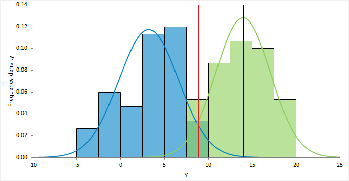
Limit of blank (also known as the critical value) is the highest quantity value that is likely to be observed, with a stated probability, for a blank material.


blank histogram

Limit of detection (LoD)

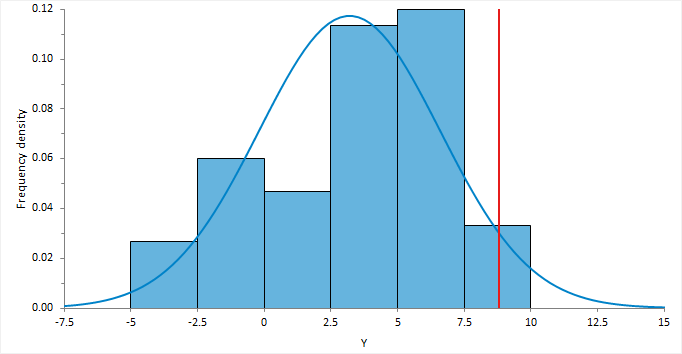
Limit of detection (also known as the minimum detectable value) is the quantity value, for which the probability of falsely claiming the absence of a measurand in a material is beta, given probability (alpha) of falsely claiming its presence.


bi histogram

Estimating the detection limit of a measurement system

Estimate the limit of detection of a measurement system or procedure.

  1. Select a cell in the dataset.
  2. On the Analyse-it ribbon tab, in the Statistical Analyses group, click Precision and then click Detection Capability.
    The analysis task pane opens.
  3. In the Y drop-down list, select the measured variable.
  4. In the By drop-down list, select the level variable, and then:
    • If the values are identifiers, select the Identifier, and then in the Assigned values grid, under the Value column alongside each level, type the value.
    • If the values are dilutions made by diluting a high pool or mixing high and low pools, select the Relationship, and then select Mixture, Dilution, or Addition based on how the levels were prepared. In the Assigned values grid, under the Value column for the first and/or last level, type the value (intermediate values are automatically calculated using relative values).
    • If the values are known/expected/assigned values, select the Known values.
    Note: Computation of detection limits only requires the assigned value of 0 for blank materials. You do not need to assign values to other materials.
  5. In the LoB Estimator drop-down list, select:
    Option Description
    Normal quantile Estimate the LoB using the 5% upper of the distribution of blank values (levels with assigned value 0).

    Use when values are normally distributed and not truncated at 0.

    Quantile Estimate the LoB using the 95th percentile of the distribution of blank values.

    Use when values are truncated at zero.

    Known value Use specific value as the LoB.
  6. In the Alpha edit box, type the probability that a blank material gives a result greater than the critical value (LoB), when in fact the substance is not present (typically 5%).
  7. In the Beta edit box, type the probability that a non-blank material gives a result less than the critical value (LoB) when in fact the substance is present (typically 5%).
  8. Click Calculate.

Estimating the detection limit using a precision profile

Estimate the limit of detection of a measurement system or procedure using a precision profile variance function.

You must have already completed the task:
  1. Activate the analysis report worksheet.
  2. On the Analyse-it ribbon tab, in the MSA group, click Detection Capability.
    The analysis task pane Detection Capability panel opens.
  3. In the LoB Estimator drop-down list, select:
    Option Description
    Normal quantile Estimate the LoB using the 5% upper of the distribution of blank values (levels with assigned value 0).

    Use when values are normally distributed and not truncated at 0.

    Quantile Estimate the LoB using the 95th percentile of the distribution of blank values.

    Use when values are truncated at zero.

    Known value Use specific value as the LoB.
  4. If you selected Normal quantile, in the SD drop-down list, select:
    Option Description
    Blank material Estimate based on material assigned a value of 0.
    Precision profile at blank material value Estimate based on the precision profile variance function at the mean value of the material assigned a value of 0.
    Precision profile at zero Estimate based on the precision profile variance function at the value 0.

    Use when it is not possible to obtain blank material, but the profile function is representative of values near zero.

  5. In the Alpha edit box, type the probability that a blank material gives a result greater than the critical value (LoB), when in fact the substance is not present (typically 5%).
  6. In the SD drop-down list, select Precision profile function.
  7. In the Beta edit box, type the probability that a non-blank material gives a result less than the critical value (LoB) when in fact the substance is present (typically 5%).
  8. Click Calculate.

Estimating the detection limit using a probit fit

Fit a probit regression model to estimate the limit of detection.

  1. Select a cell in the dataset.
  2. On the Analyse-it ribbon tab, in the Statistical Analyses group, click Fit Model, and then click Probit.
    The analysis task pane opens.
  3. In the Y drop-down list, select the binary response variable.
  4. In the Event drop-down list, select the positive outcome.
  5. In the X drop-down list, select the level variable.
  6. Next to the X drop-down list, click the drop-down menu, and then in the Transform drop-down list, select Log 10
  7. In the Plot drop-down list, select Scaled - X against Y.
  8. Clear the Individual check box, and select the Aggregate check box.
  9. On the Analyse-it ribbon tab, in the Fit Model group, click Predict, and then click X given Probability.
  10. On the analysis task pane, in the Fit panel, in the Predict X given Probability edit box, type 0.95
  11. Click Calculate.
On the analysis report, in the Predict X for Given Probability section, the predicted level at 0.95 probability is the limit of detection.

Limit of quantitation (LoQ)

Limit of quantitation is the smallest quantity value that meets the requirements for intended use.

There is no set procedure to determine the limit of quantitation. Some authors suggest setting separate goals for bias and imprecision. Others such as Westgard use a model to combine the bias and imprecision into "total error" and compare it to a total allowable error goal. Others prefer to avoid the use of models and estimate total error directly using difference between the results of a method and a reference method (Krouwer, 2002). In other areas such as immunoassays the limit of quantitation is often defined as functional sensitivity where the precision profile function CV is equal 20%.

Study design

Measurement systems analysis study requirements and dataset layout.

Requirements

  • A quantitative variable.
  • 1 or more optional factor variables indicating the random effects of interest.
  • At least 2 replicates at each level.

Dataset layout

Use a column for the measured variable (Measured value) and optionally a by variable (Level); each row is a separate measurement.

Level (optional) Measured value
120 121
120 118
120 124
120 120
120 116
240 240
240 246
240 232
240 241
240 240

Dataset layout for 1 random factor

Use a column for the measured variable (Measured value), and 1 columns for the random factor (Run), and optionally a by variable (Level); each row is a separate measurement.

Level (optional) Run Measured value
120 1 121
120 1 118
120 1
120 2 120
120 2 116
120 2
120 3
120
240 1 240
240 1 242
240 1
240 2 260
240 2 238
240 2
240 3
240

Dataset layout for 2 random factors

Use a column for the measured variable (Measured value), and 2 columns for the random factors (Day, Run), and optionally a by variable (Level); each row is a separate measurement.

Level (optional) Day Run Measured value
120 1 1 121
120 1 1 118
120 1 1
120 1 2 120
120 1 2 116
120 1 2
120 1 3
120 1
120 2 1 124
120 2 1 119
120 2 1
120 2 2 118
120 2 2 121
120 2 2
120 2 3
120 2
 

Alternate dataset layout

Use multiple columns for the replicates of the measured variable (Measured value) and a by variable (Level), each row is a separate combination of level and factors.

Level Measured value
1 0.7 0.9
2 4.6 4.1
3 6.5 6.9
4 11 12.2
Note: All the above dataset layouts can arrange replicate measurements in a single row rather than in multiple rows.

Statistical Reference Guide v6.15