
Compare Pairs examines related samples and makes inferences about the differences between them.
Related samples occur when observations are made on the same set of items or subjects at different times, or when another form of matching has occurred. If the knowing the values in one sample could tell you something about the values in the other sample, then the samples are related.
There are a few different study designs that produce related data. A paired study design takes individual observations from a pair of related subjects. A repeat measures study design takes multiple observations on the same subject. A matched pair study design takes individual observations on multiple subjects that are matched on other covariates. The purpose of matching similar subjects is often to reduce or eliminate the effects of a confounding factor.
A difference plot shows the differences between two observations on the same sampling unit.
The difference plot shows the difference between two observations on the vertical axis against the average of the two observations on the horizontal axis. A gray identity line represents equality; no difference.
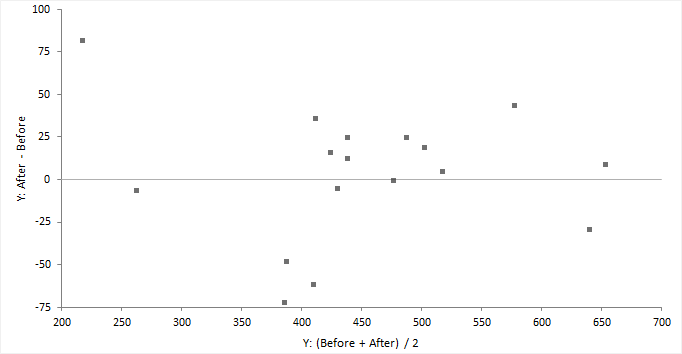
If the second observation is always greater than the first the points lie above the line of equality, or vice-versa. If differences are not related to the magnitude the points will form a horizontal band. If the points form an increasing, decreasing, or non-constant width band, then the variance is not constant.
It is common to combine the difference plot with a histogram and a normality plot of the differences to check if the differences are normally distributed, which is an assumption of some statistical tests and estimators.
Summarize the differences between two related observations.
An equality hypothesis test formally tests if two or more population means/medians are different.
Inferences about related samples are complicated by the fact that the observations are correlated. Therefore the tests for independent samples are of no use. Instead, tests for related samples focus on the differences within each sampling unit.
When the test p-value is small, you can reject the null hypothesis and conclude that the populations differ in means/medians.
An equivalence hypothesis test formally tests if two population means are equivalent, that is, practically the same.
An equality hypothesis test can never prove that the means are equal, it can only ever disprove the null hypothesis of equality. It is therefore of interest when comparing say a new treatment against a placebo, where the null hypothesis (assumption of what is true without evidence to the contrary) is that the treatment has no effect, and you want to prove the treatment produces a useful effect. By contrast, an equivalence hypothesis test is of interest when comparing say a generic treatment to an existing treatment where the aim is to prove that they are equivalent, that is the difference is less than some small negligible effect size. A equivalence hypothesis test therefore constructs the null hypothesis of non-equivalence and the goal is to prove the means are equivalent.
The null hypothesis states that the means are not equivalent, against the alternative hypothesis that the difference between the means is within the bounds of the equivalence interval, that is, the effect size is less than some small difference that is considered practically zero. The hypothesis is tested as a composite of two one-sided t-tests (TOST), H01 tests the hypothesis that mean difference is less than the lower bound of the equivalence interval, test H02 that the mean difference is greater than the upper bounds of the equivalence interval. The p-value is the greater of the two one-sided t-test p-values. When the test p-value is small, you can reject the null hypothesis and conclude the samples are from populations with practically equivalent means.
Tests for the equality of means/medians of related samples and their properties and assumptions.
| Test | Purpose |
|---|---|
| Z | Test if the difference between means is equal to a hypothesized value when the population standard deviation is known. Assumes the population differences are normally distributed. Due to the central limit theorem, the test may still be useful when this assumption is not true if the sample size is moderate. However, in this case, the Wilcoxon test may be more powerful. |
| Student's t | Test if the difference between means is equal to a hypothesized value. Assumes the population differences are normally distributed. Due to the central limit theorem, the test may still be useful when this assumption is not true if the sample size is moderate. However, in this case, the Wilcoxon test may be more powerful. |
| Wilcoxon | Test if there is a shift in location equal to the hypothesized value. Under the assumption that the population distribution of the differences is symmetric, the hypotheses can be stated in terms of a difference between means/medians. Under the less strict hypotheses, requiring no distributional assumptions, the hypotheses can be stated as the probability that the sum of a randomly chosen pair of differences exceeds zero is 0.5. |
| Sign | Test if the median of the differences is equal to a hypothesized value. Under the more general hypotheses, tests if given a random pair of observations (xi, yi), that xi and yi are equally likely to be larger than the other. Has few assumptions, but lacks power compared to the Wilcoxon and Student's t test. |
| TOST (two-one-sided t-tests) | Test if the means are equivalent. Assumes the populations are normally distributed. Due to the central limit theorem, the test may still be useful when this assumption is not true if the sample sizes are equal, moderate size, and the distributions have a similar shape. |
| ANOVA | Test if the two or means are equal. Assumes the populations are normally distributed. Due to the central limit theorem, the test may still be useful when the assumption is violated if the sample sizes are equal and moderate size. However, in this situation the Friedman test is may be more powerful. |
| Friedman | Test if two or medians are equal. Has few assumptions, and is equivalent to a two-sided Sign test in the case of two samples. |
Test if there is a difference between the means/medians of two or more related samples.
Test if there is equivalence of means of two related samples.
An effect size estimates the magnitude of the difference between two means/medians.
The term effect size relates to both unstandardized measures (for example, the difference between group means) and standardized measures (such as Cohen's d; the standardized difference between group means). Standardized measures are more appropriate than unstandardized measures when the metrics of the variables do not have intrinsic meaning, when combining results from multiple studies, or when comparing results from studies with different measurement scales.
A point estimate is a single value that is the best estimate of the true unknown parameter; a confidence interval is a range of values and indicates the uncertainty of the estimate.
Estimators for the difference in means/medians of related samples and their properties and assumptions.
| Estimator | Purpose |
|---|---|
| Mean difference | Estimate the difference between the means. |
| Standardized mean difference | Estimate the standardized difference between the means. Cohen's d is the most popular estimator using the difference between the means divided by the pooled sample standard deviation. Cohen's d is a biased estimator of the population standardized mean difference (although the bias is very small and disappears for moderate to large samples) whereas Hedge's g applies an unbiasing constant to correct for the bias. |
| Median difference | Estimate the median of the differences. |
| Hodges-Lehmann location shift | Estimate the shift in location. A shift in location is equivalent to a difference between means/medians when the distribution of the differences is symmetric. Symmetry is quite often inherently satisfied for paired data. |
Estimate the difference between the means/medians of 2 related samples.
Compare pairs analysis study requirements and dataset layout.
Use a column for each response variable (Blood pressure - Before, Blood pressure - After); each row has the values of the variables for a case (Subject).
| Blood pressure | ||
|---|---|---|
| Subject (optional) | Before | After |
| 1 | 123 | 124 |
| 2 | 109 | 97 |
| 3 | 112 | 113 |
| 4 | 102 | 105 |
| 5 | 98 | 95 |
| 6 | 114 | 119 |
| 7 | 119 | 114 |
| 8 | 112 | 114 |
| 9 | 110 | 121 |
| 10 | 117 | 118 |
| … | … | … |
Use a column the response variable (Blood pressure), a column for the factor variable (Intervention), and a column for the blocking variable (Pair); each row has the values of the variables for a case.
| Pair | Intervention | Blood pressure |
|---|---|---|
| 1 | Before | 123 |
| 2 | Before | 109 |
| 3 | Before | 112 |
| 4 | Before | 102 |
| 5 | Before | 98 |
| 6 | Before | 114 |
| 7 | Before | 119 |
| 8 | Before | 112 |
| 9 | Before | 110 |
| 10 | Before | 117 |
| … | Before | … |
| 1 | After | 124 |
| 2 | After | 97 |
| 3 | After | 113 |
| 4 | After | 105 |
| 5 | After | 95 |
| 6 | After | 119 |
| 7 | After | 114 |
| 8 | After | 114 |
| 9 | After | 121 |
| 10 | After | 118 |
| … | After | … |


