
Precision is the closeness of agreement between measured quantity values obtained by replicate measurements on the same or similar objects under specified conditions.
Precision is not a quantity and therefore it is not expressed numerically. Rather, it is expressed by measures such as the variance, standard deviation, or coefficient of variation under the specified conditions of measurement
Many different factors may contribute to the variability between replicate measurements, including the operator; the equipment used; the calibration of the equipment; the environment; the time elapsed between measurements.
Two conditions of precision, termed repeatability and reproducibility conditions are useful for describing the variability of a measurement procedure. Other intermediate conditions between these two extreme conditions of precision are also conceivable and useful, such as conditions within a single laboratory.
Reproducibility is a measure of precision under a defined set of conditions: different locations, operators, measuring systems, and replicate measurements on the same or similar objects.
Intermediate precision (also called within-laboratory or within-device) is a measure of precision under a defined set of conditions: same measurement procedure, same measuring system, same location, and replicate measurements on the same or similar objects over an extended period of time. It may include changes to other conditions such as new calibrations, operators, or reagent lots.
Repeatability (also called within-run precision) is a measure of precision under a defined set of conditions: same measurement procedure, same operators, same measuring system, same operating conditions and same location, and replicate measurements on the same or similar objects over a short period of time.
Variance components are estimates of a part of the total variability accounted for by a specified source of variability.
Random factors are factors where a number of levels are randomly sampled from the population, and the intention is to make inferences about the population. For example, a study might examine the precision of a measurement procedure in different laboratories. In this case, there are 2 variance components: variation within an individual laboratory and the variation among all laboratories. When performing the study it is impractical to study all laboratories, so instead a random sample of laboratories are used. More complex studies may examine the precision within a single run, within a single laboratory, and across laboratories.
Most precision studies use a nested (or hierarchical) model where each level of a nested factor is unique amongst each level of the outer factor. The basis for estimating the variance components is the nested analysis of variance (ANOVA). Estimates of the variance components are extracted from the ANOVA by equating the mean squares to the expected mean squares. If the variance is negative, usually due to a small sample size, it is set to zero. Variance components are combined by summing them to estimate the precision under different conditions of measurements.
The variance components can be expressed as a variance, standard deviation (SD), or coefficient of variation (CV). A point estimate is a single value that is the best estimate of the true unknown parameter; a confidence interval is a range of values and indicates the uncertainty of the estimate. A larger estimate reflects less precision.
| Estimator | Description |
|---|---|
| Exact | Used to form intervals on the inner-most nested variance components. Based on the F-distribution. |
| Satterthwaite | Used to form intervals on the sum of the variances. Based on the F-distribution, as above, but uses modified degrees of freedom. Works well when the factors have equal or a large number of levels, though when the differences between them are large it can produce unacceptably liberal confidence intervals. |
| Modified Large Sample (MLS) | Used to form intervals on the sum of variances or individual components. A modification of the large sample normal theory approach to constructing confidence intervals. Provides good coverage close to the nominal level in a wide range of cases. |
Estimate the precision of a measurement system or procedure.
Test if the precision matches a performance claim.
You should use this procedure when you already have a performance claim from a manufacturer's package insert, and you want to test whether your precision is significantly greater than the claim. It is possible for the precision from a study to be greater than the claim, but for the difference to be due to the random error in your study.
A precision profile plot shows precision against the measured quantity value over the measuring interval.
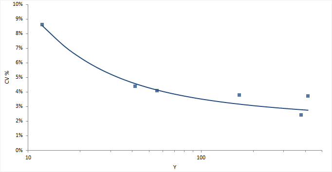
Plot a precision profile to observe the performance over the entire measuring interval.
A variance function describes the relationship between the variance and the measured quantity value.
| Fit | Description |
|---|---|
| Constant variance | Fit constant variance across the measuring interval. |
| Constant CV | Fit constant coefficient of variation across the measuring interval. |
| Mixed constant / proportional variance | Fit constant variance at low levels with constant coefficient of variation at high levels. |
| 2-parameter | Fir a 2-parameter linear variance function. |
| 3-parameter | Fit Sadler 3-parameter variance function – a monotone relationship (either increasing or decreasing) between the variance and level of measurement. |
| 3-parameter alternative | Fit Sadler alternate 3-parameter variance function – gives more flexibility than the Sadler standard 3-parameter variance function especially near zero. |
| 4-parameter | Fit a Sadler 4-parameter variance function - allows for a turning point near the detection limit. |
A variance function can be useful to estimate the limit of detection or limit of quantitation.
Plot a precision profile to observe the performance over the entire measuring interval.
Measurement systems analysis study requirements and dataset layout.
Use a column for the measured variable (Measured value) and optionally a by variable (Level); each row is a separate measurement.
| Level (optional) | Measured value |
|---|---|
| 120 | 121 |
| 120 | 118 |
| 120 | 124 |
| 120 | 120 |
| 120 | 116 |
| … | … |
| 240 | 240 |
| 240 | 246 |
| 240 | 232 |
| 240 | 241 |
| 240 | 240 |
| … | … |
Use a column for the measured variable (Measured value), and 1 columns for the random factor (Run), and optionally a by variable (Level); each row is a separate measurement.
| Level (optional) | Run | Measured value |
|---|---|---|
| 120 | 1 | 121 |
| 120 | 1 | 118 |
| 120 | 1 | … |
| 120 | 2 | 120 |
| 120 | 2 | 116 |
| 120 | 2 | … |
| 120 | 3 | … |
| 120 | … | … |
| … | … | … |
| 240 | 1 | 240 |
| 240 | 1 | 242 |
| 240 | 1 | … |
| 240 | 2 | 260 |
| 240 | 2 | 238 |
| 240 | 2 | … |
| 240 | 3 | … |
| 240 | … | … |
| … | … | … |
Use a column for the measured variable (Measured value), and 2 columns for the random factors (Day, Run), and optionally a by variable (Level); each row is a separate measurement.
| Level (optional) | Day | Run | Measured value |
|---|---|---|---|
| 120 | 1 | 1 | 121 |
| 120 | 1 | 1 | 118 |
| 120 | 1 | 1 | … |
| 120 | 1 | 2 | 120 |
| 120 | 1 | 2 | 116 |
| 120 | 1 | 2 | … |
| 120 | 1 | 3 | … |
| 120 | 1 | … | … |
| 120 | 2 | 1 | 124 |
| 120 | 2 | 1 | 119 |
| 120 | 2 | 1 | … |
| 120 | 2 | 2 | 118 |
| 120 | 2 | 2 | 121 |
| 120 | 2 | 2 | … |
| 120 | 2 | 3 | … |
| 120 | 2 | … | … |
| … | … | … |
Use multiple columns for the replicates of the measured variable (Measured value) and a by variable (Level), each row is a separate combination of level and factors.
| Level | Measured value | ||
|---|---|---|---|
| 1 | 0.7 | 0.9 | … |
| 2 | 4.6 | 4.1 | … |
| 3 | 6.5 | 6.9 | … |
| 4 | 11 | 12.2 | … |

