Contingency tables

Contingency analysis describes and visualizes the distribution of categorical variables, and makes inferences about the equality of proportions, independence of the variables, or agreement between variables.

• Contingency table
  A contingency table, also known as a cross-classification table, describes the relationships between two or more categorical variables.
• Grouped frequency plot
  A grouped or stacked frequency plot shows the joint or conditional distributions.
• Effect size
  An effect size estimates the magnitude of the difference of proportions or the association between two categorical variables.
• Relative risk
  Relative risk is the ratio of the probability of the event occurring in one group versus another group.
• Inferences about equality of proportions
  Inferences about the proportions in populations are made using random samples of data drawn from each population of interest.
• Inferences about independence
  Inferences about the independence between categorical variables are made using a random bivariate sample of data drawn from the population of interest.
• Mosaic plot
  A mosaic plot is a visual representation of the association between two variables.

A contingency table, also known as a cross-classification table, describes the relationships between two or more categorical variables.

A table cross-classifying two variables is called a 2-way contingency table and forms a rectangular table with rows for the R categories of the X variable and columns for the C categories of a Y variable. Each intersection is called a cell and represents the possible outcomes. The cells contain the frequency of the joint occurrences of the X, Y outcomes. A contingency table having R rows and C columns is called an R x C table.

A variable having only two categories is called a binary variable. When both variables are binary, the resulting contingency table is a 2 x 2 table. Also, commonly known as a four-fold table because there are four cells.

A contingency table can summarize three probability distributions – joint, marginal, and conditional.

• The joint distribution describes the proportion of the subjects jointly classified by a category of X and a category of Y. The cells of the contingency table divided by the total provides the joint distribution. The sum of the joint distribution is 1.
• The marginal distributions describe the distribution of the X (row) or Y (column) variable alone. The row and column totals of the contingency table provide the marginal distributions. The sum of a marginal distribution is 1.
• The conditional distributions describe the distribution of one variable given the levels of the other variable. The cells of the contingency table divided by the row or column totals provide the conditional distributions. The sum of a conditional distribution is 1.

When both variables are random, you can describe the data using the joint distribution, the conditional distribution of Y given X, or the conditional distribution of X given Y.

When one variable is and explanatory variable (X, fixed) and the other a response variable (Y, random), the notion of a joint distribution is meaningless, and you should describe the data using the conditional distribution of Y given X. Likewise, if Y is a fixed variable and X random, you should describe the data using the conditional distribution of X given Y.

When the variables are matched-pairs or repeated measurements on the same sampling unit, the table is square R=C, with the same categories on both the rows and columns. For these tables, the cells may exhibit a symmetric pattern about the main diagonal of the table, or the two marginal distributions may differ in some systematic way.

Cross-classify data into a 2-way contingency table.

1. Select a cell in the dataset.
2. On the Analyse-it ribbon tab, in the Statistical Analyses group, click Compare Groups, and then click Contingency table.
   The analysis task pane opens.
3. In the Y drop-down list, select the first categorical variable.
4. In the X drop-down list, select the second categorical variable.
5. If the data are in frequency form, in the Frequency drop-down list, select the frequency count variable.
6. Optional: To customize the statistics to show, click Customize... and then select or clear the appropriate check boxes. To save the options as the default to show for all new analyses, click Save as Defaults.
7. Click Calculate.

Cross-classify related data into a 2-way contingency table.

1. Select a cell in the dataset.
2. On the Analyse-it ribbon tab, in the Statistical Analyses group, click Compare Pairs, and then click Contingency Table.
   The analysis task pane opens.
3. If the data consists of paired/repeated measurements in separate variables:
   1. In the Model drop-down menu, select Paired / Repeated.
   2. In the Y lists, select two categorical variables.
4. If the data consist of matched pairs with a separate response variable, factor variable, and blocking variable:
   1. In the Model drop-down menu, select Matched.
   2. In the Y drop-down list, select the categorical response variable.
   3. In the X (factor) drop-down list, select the categorical factor variable identifying the groups.
   4. In the Block drop-down list, select the blocking variable identifying the matching.
5. If the data are in frequency form, in the Frequency drop-down list, select the frequency count variable.
6. Optional: To customize the statistics to show, click Customize... and then select or clear the appropriate check boxes. To save the options as the default to show for all new analyses, click Save as Defaults.
7. Click Calculate.

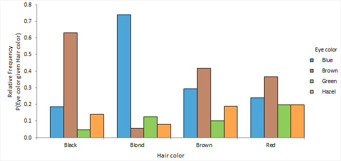
A grouped or stacked frequency plot shows the joint or conditional distributions.

An effect size estimates the magnitude of the difference of proportions or the association between two categorical variables.

A point estimate is a single value that is the best estimate of the true unknown parameter; a confidence interval is a range of values and indicates the uncertainty of the estimate.

For tables larger than 2 x 2, you must partition the contingency table into a series of 2 x 2 sub-tables to estimate the effect size.

Estimators for contingency tables and their properties and assumptions.

Estimate the odds ratio.

1. Select a cell in the dataset.
2. On the Analyse-it ribbon tab, in the Statistical Analyses group, click Compare Groups, and then click Odds Ratio.
   The analysis task pane opens.
3. In the Y drop-down list, select the first categorical variable.
4. In the X drop-down list, select the second categorical variable.
5. If the data are in frequency form, in the Frequency drop-down list, select the frequency count variable.
6. In the Ratio drop-down list, select the ratio of interest, and in the Event drop-down list, select the outcome of interest.
7. In the Confidence interval edit box, type the confidence level as a percentage, or type - to suppress the confidence interval, and then in the drop-down list, select the confidence bounds.
8. In the Method drop-down list, select the interval estimator.
9. Click Calculate.

Estimate the odds ratio for related data.

1. Select a cell in the dataset.
2. On the Analyse-it ribbon tab, in the Statistical Analyses group, click Compare Pairs, and then click Odds Ratio.
   The analysis task pane opens.
3. If the data consists of paired/repeated measurements in separate variables:
   1. In the Model drop-down menu, select Paired / Repeated.
   2. In the Y lists, select two categorical variables.
4. If the data consist of matched pairs with a separate response variable, factor variable, and blocking variable:
   1. In the Model drop-down menu, select Matched.
   2. In the Y drop-down list, select the categorical response variable.
   3. In the X (factor) drop-down list, select the categorical factor variable identifying the groups.
   4. In the Block drop-down list, select the blocking variable identifying the matching.
5. If the data are in frequency form, in the Frequency drop-down list, select the frequency count variable.
6. In the Ratio drop-down list, select the ratio of interest, and in the Event drop-down list, select the outcome of interest.
7. In the Confidence interval edit box, type the confidence level as a percentage, or type - to suppress the confidence interval, and then in the drop-down list, select the confidence bounds.
8. In the Method drop-down list, select the interval estimator.
9. Click Calculate.

Relative risk is the ratio of the probability of the event occurring in one group versus another group.

Medical statistics uses categorical data analysis extensively to describe the association between the occurrence of a disease and exposure to a risk factor. In this application, the terminology is often used to frame the statistics in terms of risk. Risk difference is equivalent to a difference between proportions, and a risk ratio is equivalent to a ratio of proportions.

The term relative risk is the ratio of the probability of the event occurring in the exposed group versus a non-exposed group. It is the same as the risk ratio. Although a relative risk is different from odds ratio, in some circumstances, such as the low prevalence of the disease, the odds ratio asymptotically approaches the relative risk and is, therefore, an estimate of the relative risk. It is better to avoid confusion and use the terms risk ratio and odds ratio for the effect size estimates and use the term relative risk for the population parameter.

A prospective cohort study or a clinical trial can estimate the risk ratio or the odds ratio of the occurrence of a disease given exposure to a risk factor. Whereas, a retrospective case-control study can estimate the odds ratio of the risk factor given the disease, which is equivalent to the odds ratio of the occurrence of the disease given the risk factor. A risk ratio is not useful because it refers to the risk factor given the disease, which is not normally of interest. However, as stated above the odds ratio can be used as an estimate of the relative risk in most circumstances.

Practitioners often prefer the risk ratio due to its more direct interpretation. Statisticians tend to prefer the odds ratio as it applies to a wide range of study designs, allowing comparison between different studies and meta-analysis based on many studies.  It also forms the basis of logistic regression.

Inferences about the proportions in populations are made using random samples of data drawn from each population of interest.

• Equality of proportions hypothesis test
  A hypothesis test formally tests if the proportions in two or more populations are equal.
• Exact and asymptotic p-values
  Asymptotic p-values are useful for large sample sizes when the calculation of an exact p-value is too computer-intensive.
• Wald, Score, Likelihood ratio
  Three different ways are used to make large sample inferences all using a X² statistic, so it is important to understand the differences to avoid confusion.

A hypothesis test formally tests if the proportions in two or more populations are equal.

When one variable is an explanatory variable (X, fixed) and the other a response variable (Y, random), the hypothesis of interest is whether the populations have the same or different proportions in each category.

When the test p-value is small, you can reject the null hypothesis and conclude that the populations differ in the proportions in at least one category.

Tests for contingency tables larger than 2 x 2 are omnibus tests and do not tell you which groups differ from each other or in which categories. You should use the mosaic plot to examine the association, or partition the contingency table into a series of 2 x 2 sub-tables and test each table.

Asymptotic p-values are useful for large sample sizes when the calculation of an exact p-value is too computer-intensive.

Many test statistics follow a discrete probability distribution. However, hand calculation of the true probability distributions of many test statistics is too tedious except for small samples. It can be computationally difficult and time intensive even for a powerful computer. Instead, many statistical tests use an approximation to the true distribution. Approximations assume the sample size is large enough so that the test statistic converges to an appropriate limiting normal or chi-square distribution.

A p-value that is calculated using an approximation to the true distribution is called an asymptotic p-value. A p-value calculated using the true distribution is called an exact p-value. For large sample sizes, the exact and asymptotic p-values are very similar. For small sample sizes or sparse data, the exact and asymptotic p-values can be quite different and can lead to different conclusions about the hypothesis of interest.

When using the true distribution, due to the discreteness of the distribution, the p-value and confidence intervals are conservative. A conservative interval guarantees that the actual coverage level is at least as large as the nominal confidence level, though it can be much larger. For a hypothesis test, it guarantees protection from type I error at the nominal significance level. Some statisticians prefer asymptotic p-values and intervals, as they tend to achieve an average coverage closer to the nominal level. The problem is the actual coverage of a specific test or interval may be less than the nominal level.

Although a statistical test might commonly use an approximation, it does not mean it cannot be calculated using the true probability distribution. For example, an asymptotic p-value for the Pearson X² test uses the chi-squared approximation, but the test could also compute an exact p-value using the true probability distribution. Similarly, although the Fisher test is often called the Fisher exact test because it computes an exact p-value using the hypergeometric probability distribution, the test could also compute an asymptotic p-value. Likewise, the Wilcoxon-Mann-Whitney test often computes an exact p-value for small sample sizes and reverts to an asymptotic p-value for large sample sizes.

Three different ways are used to make large sample inferences all using a X² statistic, so it is important to understand the differences to avoid confusion.

The score, likelihood ratio, and Wald evidence functions are useful when analyzing categorical data. All have approximately chi-squared (X²) distribution when the sample size is sufficiently large.

Because of their underlying use of the X² distribution, mixing of the techniques often occurs when testing hypotheses and constructing interval estimates. Introductory textbooks often use a score evidence function for the hypothesis test then use a Wald evidence function for the confidence interval. When you use different evidence functions the results can be inconsistent. The hypothesis test may be statistically significant, but the confidence interval may include the hypothesized value suggesting the result is not significant. Where possible you should use the same underlying evidence function to form the confidence interval and test the hypotheses.

Note that when the degrees of freedom is 1 the Pearson X² statistic is equivalent to a squared score Z statistic because they are both based on the score evidence function. A 2-tailed score Z test produces the same p-value as a Pearson X² test.

Many Wald-based interval estimates have poor coverage and defy conventional wisdom. Modern computing power allows the use of computationally intensive score evidence functions for interval estimates, such that we recommended them for general use.

Tests for the equality of proportions of independent samples and their properties and assumptions.

Test if there is a difference between the proportions of two or more independent samples.

1. Select a cell in the dataset.
2. On the Analyse-it ribbon tab, in the Statistical Analyses group, click Compare Groups, and then click the hypothesis test.
   The analysis task pane opens.
3. In the Y drop-down list, select the categorical response variable.
4. In the X drop-down list, select the categorical factor variable that identifies the groups.
5. If the data are in frequency form, in the Frequency drop-down list, select the frequency count variable.
6. In the Hypotheses drop-down list, select the null and alternative hypothesis.
7. Optional: To compare the p-value against a predefined significance level, in the Significance level edit box, type the maximum probability of rejecting the null hypothesis when in fact it is true (typically 5% or 1%).
8. Click Calculate.

Tests for the equality of proportions of related samples and their properties and assumptions.

Test if there is a difference between the proportions of two or more related samples.

1. Select a cell in the dataset.
2. On the Analyse-it ribbon tab, in the Statistical Analyses group, click Compare Pairs, and then click the hypothesis test.
   The analysis task pane opens.
3. If the data consists of paired/repeated measurements in separate variables:
   1. In the Model drop-down menu, select Paired / Repeated.
   2. In the Y lists, select two categorical variables.
4. If the data consist of matched pairs with a separate response variable, factor variable, and blocking variable:
   1. In the Model drop-down menu, select Matched.
   2. In the Y drop-down list, select the categorical response variable.
   3. In the X (factor) drop-down list, select the categorical factor variable identifying the groups.
   4. In the Block drop-down list, select the blocking variable identifying the matching.
5. If the data are in frequency form, in the Frequency drop-down list, select the frequency count variable.
6. In the Hypotheses drop-down list, select the null and alternative hypothesis.
7. Optional: To compare the p-value against a predefined significance level, in the Significance level edit box, type the maximum probability of rejecting the null hypothesis when in fact it is true (typically 5% or 1%).
8. Click Calculate.

Inferences about the independence between categorical variables are made using a random bivariate sample of data drawn from the population of interest.

• Independence hypothesis test
  A hypothesis test formally tests whether 2 categorical variables are independent.
• Continuity correction
  Continuity corrections such as Yates X²are no longer needed with modern computing power.

A hypothesis test formally tests whether 2 categorical variables are independent.

When both variables are random, the hypothesis of interest is whether the variables are independent.

The null hypothesis states that the variables are independent, against the alternative hypothesis that the variables are not independent. That is, in terms of the contingency table, the null hypothesis states the event "an observation is in row i" is independent of the event "that same observation is in column j," for all i and j, against the alternative hypothesis that is the negation of the null hypothesis.

When the test p-value is small, you can reject the null hypothesis and conclude that the variables are not independent.

Continuity corrections such as Yates X²are no longer needed with modern computing power.

Continuity corrections have historically been used to make adjustments to the p-value when a continuous distribution approximates a discrete distribution. Yates correction for the Pearson chi-square (X²) test is probably the most well-known continuity correction. In some cases, the continuity correction may adjust the p-value too far, and the test then becomes overly conservative.

Modern computing power makes such corrections unnecessary, as exact tests that use the discrete distributions are available for moderate and in many cases even large sample sizes. Hirji (Hirji 2005), states "An applied statistician today, in our view, may regard such corrections as interesting historical curiosities."

Tests for the independence of 2 categorical variables and their properties and assumptions.

Test if two categorical variables are independent in a bivariate population represented by the sample.

1. Select a cell in the dataset.
2. On the Analyse-it ribbon tab, in the Statistical Analyses group, click Compare Groups, and then click the hypothesis test.
   The analysis task pane opens.
3. In the X and Y drop-down lists, select the categorical variables.
4. In the Hypotheses drop-down list, select the independence null and alternative hypotheses (the 2nd in the list).
5. Optional: To compare the p-value against a predefined significance level, in the Significance level edit box, type the maximum probability of rejecting the null hypothesis when in fact it is true (typically 5% or 1%).
6. Click Calculate.

A mosaic plot is a visual representation of the association between two variables.

A mosaic plot is a square subdivided into rectangular tiles the area of which represents the conditional relative frequency for a cell in the contingency table. Each tile is colored to show the deviation from the expected frequency (residual) from a Pearson X² or Likelihood Ratio G² test.

You can use the mosaic plot to discover the association between two variables. Red tiles indicate significant negative residuals, where the frequency is less than expected. Blue tiles indicate significant positive residuals, where the frequency is greater than expected. The intensity of the color represents the magnitude of the residual.

Visualize the association between 2 categorical variables.

1. Select a cell in the dataset.
2. On the Analyse-it ribbon tab, in the Statistical Analyses group, click Compare Groups, and then click Mosaic.
   The analysis task pane opens.
3. In the Y drop-down list, select the categorical response variable.
4. In the X drop-down list, select the categorical factor variable identifying the groups.
5. In the Color by drop-down list, select Category to color by category, or Residual to color by the Pearson X² residual.
6. To label the tiles with the conditional relative frequency, click Label tiles.
7. Click Calculate.

Contingency analysis study requirements and dataset layout.