Compare groups

Compare Groups examines independent samples and makes inferences about the differences between them.

Independent samples occur when observations are made on different sets of items or subjects. If the values in one sample do not tell you anything about the values in the other sample, then the samples are independent. If the knowing the values in one sample could tell you something about the values in the other sample, then the samples are related.

• Side-by-side univariate plots
  Side-by-side univariate plots summarize the distribution of data stratified into groups.
• Equality of means/medians hypothesis test
  An equality hypothesis test formally tests if two or more population means/medians are different.
• Equivalence of means hypothesis test
  An equivalence hypothesis test formally tests if two population means are equivalent, that is, practically the same.
• Difference between means/medians effect size
  An effect size estimates the magnitude of the difference between two means/medians.
• Multiple comparisons
  Multiple comparisons make simultaneous inferences about a set of parameters.
• Mean-Mean scatter plot
  A mean-mean scatter plot shows a 2-dimensional representation of the differences between many means.
• Homogeneity of variance hypothesis test
  A homogeneity hypothesis test formally tests if the populations have equal variances.

Use univariate descriptive statistics to describe a quantitative variable that is classified by a factor variable.

1. Select a cell in the dataset.
2. On the Analyse-it ribbon tab, in the Statistical Analyses group, click Compare Groups, and then click the statistics to show:

   Option	Description
   Mean and Moments	Show mean, variance, standard deviation.
   Median and Quartiles	Show minimum, maximum, median, and quartiles.

   The analysis task pane opens.
3. In the Y drop-down list, select the quantitative response variable.
4. In the X drop-down list, select the categorical factor variable identifying the groups.
5. Optional: To customize the statistics to show, click Customize... and then select or clear the appropriate check boxes. To save the options as the defaults to use for future analyses, click Save as Defaults.
6. Click Calculate.

Side-by-side univariate plots summarize the distribution of data stratified into groups.

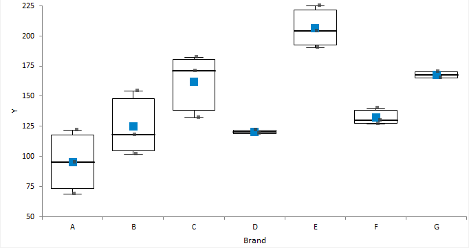
Summarize the distribution of a single quantitative variable stratified into groups.

1. Select a cell in the dataset.
2. On the Analyse-it ribbon tab, in the Statistical Analyses group, click Compare Groups > Univariate, and then click the plot type.
   The analysis task pane opens.
3. In the Y drop-down list, select the quantitative response variable.
4. In the X drop-down list, select the categorical factor variable identifying the groups.
5. Optional: To overlay more than one plot type on the same chart, on the Analyse-it ribbon tab, in the Compare Groups group, click Univariate, and then click an additional plot type.
6. Optional: In the analysis task pane, customize the options for the plot.
7. Click Calculate.

An equality hypothesis test formally tests if two or more population means/medians are different.

When the test p-value is small, you can reject the null hypothesis and conclude that the populations differ in means/medians.

Tests for more than two samples are omnibus tests and do not tell you which groups differ from each other. You should use multiple comparisons to make these inferences.

An equivalence hypothesis test formally tests if two population means are equivalent, that is, practically the same.

An equality hypothesis test can never prove that the means are equal, it can only ever disprove the null hypothesis of equality. It is therefore of interest when comparing say a new treatment against a placebo, where the null hypothesis (assumption of what is true without evidence to the contrary) is that the treatment has no effect, and you want to prove the treatment produces a useful effect. By contrast, an equivalence hypothesis test is of interest when comparing say a generic treatment to an existing treatment where the aim is to prove that they are equivalent, that is the difference is less than some small negligible effect size. A equivalence hypothesis test therefore constructs the null hypothesis of non-equivalence and the goal is to prove the means are equivalent.

The null hypothesis states that the means are not equivalent, against the alternative hypothesis that the difference between the means is within the bounds of the equivalence interval, that is, the effect size is less than some small difference that is considered practically zero. The hypothesis is tested as a composite of two one-sided t-tests (TOST), H0₁ tests the hypothesis that mean difference is less than the lower bound of the equivalence interval, test H0₂ that the mean difference is greater than the upper bounds of the equivalence interval. The p-value is the greater of the two one sided t-test p-values. When the test p-value is small, you can reject the null hypothesis and conclude the samples are from populations with practically equivalent means.

Tests for the equality/equivalence of means/medians of independent samples and their properties and assumptions.

Test if there is a difference between the means/medians of two or more independent samples.

1. Select a cell in the dataset.
2. On the Analyse-it ribbon tab, in the Statistical Analyses group, click Compare Groups, and then click the hypothesis test.
   The analysis task pane opens.
3. In the Y drop-down list, select the quantitative response variable.
4. In the X drop-down list, select the categorical factor variable identifying the groups.
5. If performing a 2 sample hypothesis test:
   1. In the Hypotheses drop-down list, select the null and directional alternative hypotheses.
   2. In the Hypothesized difference edit box, type the expected difference under the null hypothesis.
6. If performing a k sample hypothesis test:
   1. In the Hypothesis drop-down list, select the null and alternative hypotheses.
7. Optional: To compare the p-value against a predefined significance level, in the Significance level edit box, type the maximum probability of rejecting the null hypothesis when in fact it is true (typically 5% or 1%).
8. Click Calculate.

Test if there is equivalence of the means of two independent samples.

1. Select a cell in the dataset.
2. On the Analyse-it ribbon tab, in the Statistical Analyses group, click Compare Groups, and then click TOST hypothesis test.
   The analysis task pane opens.
3. In the Y drop-down list, select the quantitative response variable.
4. In the X drop-down list, select the categorical factor variable identifying the groups.
5. In the Test drop-down list, select either Student's t or Welch t depending on the homogeneity of variances.

   The TOST equivalence test is actually specified through the Hypotheses drop-down list, the Test drop-down list indicates the type of t-test to use.

6. In the Equivalence interval edit boxes, type the lower and upper bounds of the equivalence interval. For example, type-5 to +5 if differences between the means of ±5 is the effect size considered to be practically the same.
7. Optional: To compare the p-value against a predefined significance level, in the Significance level edit box, type the maximum probability of rejecting the null hypothesis when in fact it is true (typically 5% or 1%).
8. Click Calculate.

An effect size estimates the magnitude of the difference between two means/medians.

The term effect size relates to both unstandardized measures (for example, the difference between group means) and standardized measures (such as Cohen's d; the standardized difference between group means). Standardized measures are more appropriate than unstandardized measures when the metrics of the variables do not have intrinsic meaning, when combining results from multiple studies, or when comparing results from studies with different measurement scales.

A point estimate is a single value that is the best estimate of the true unknown parameter; a confidence interval is a range of values and indicates the uncertainty of the estimate.

Estimators for the difference in means/medians of independent samples and their properties and assumptions.

Estimate the difference between the means/medians of 2 independent samples.

1. Select a cell in the dataset.
2. On the Analyse-it ribbon tab, in the Statistical Analyses group, click Compare Groups, and then click the effect size estimator.
   The analysis task pane opens.
3. In the Y drop-down list, select the quantitative response variable.
4. In the X drop-down list, select the categorical factor variable identifying the groups.
5. In the Difference drop-down list, select the direction of the difference.
6. In the Confidence interval edit box, type the confidence level as a percentage, or type - to suppress the confidence interval, and then in the drop-down list, select the confidence bounds.
7. In the Method drop-down list, select the interval estimator.
8. Click Calculate.

Multiple comparisons make simultaneous inferences about a set of parameters.

When making inferences about more than one parameter (such as comparing many means, or the differences between many means), you must use multiple comparison procedures to make inferences about the parameters of interest. The problem when making multiple comparisons using individual tests such as Student's t-test applied to each comparison is the chance of a type I error increases with the number of comparisons. If you use a 5% significance level with a hypothesis test to decide if two groups are significantly different, there is a 5% probability of observing a significant difference that is simply due to chance (a type I error). If you made 20 such comparisons, the probability that one or more of the comparisons is statistically significant simply due to chance increases to 64%. With 50 comparisons, the chance increases to 92%. Another problem is the dependencies among the parameters of interest also alter the significance level. Therefore, you must use multiple comparison procedures to maintain the simultaneous probability close to the nominal significance level (typically 5%).

Multiple comparison procedures are classified by the strength of inference that can be made and the error rate controlled. A test of homogeneity controls the probability of falsely declaring any pair to be different when in fact all are the same. A stronger level of inference is confident inequalities and confident directions which control the probability of falsely declaring any pair to be different regardless of the values of the others. An even stronger level is a set of simultaneous confidence intervals that guarantees that the simultaneous coverage probability of the intervals is at least 100(1-alpha)% and also have the advantage of quantifying the possible effect size rather than producing just a p-value. A higher strength inference can be used to make an inference of a lesser strength but not vice-versa. Therefore, a confidence interval can be used to perform a confidence directions/inequalities inference, but a test of homogeneity cannot make a confidence direction/inequalities inference.

The most well known multiple comparison procedures, Bonferroni and Šidák, are not multiple comparison procedures per se. Rather they are an inequality useful in producing easy to compute multiple comparison methods of various types. In most scenarios, there are more powerful procedures available. A useful application of Bonferroni inequality is when there are a small number of pre-planned comparisons. In these cases, you can use the standard hypothesis test or confidence interval with the significance level (alpha) set to the Bonferroni inequality (alpha divided by the number of comparisons).

A side effect of maintaining the significance level is a lowering of the power of the test. Different procedures have been developed to maintain the power as high as possible depending on the strength of inference required and the number of comparisons to be made. All contrasts comparisons allow for any possible contrast; all pairs forms the k*(k-1)/2 pairwise contrasts, whereas with best forms k contrasts each with the best of the others, and against control forms k-1 contrasts each against the control group. You should choose the appropriate contrasts of interest before you perform the analysis, if you decide after inspecting the data, then you should only use all contrasts comparison procedures.

A mean-mean scatter plot shows a 2-dimensional representation of the differences between many means.

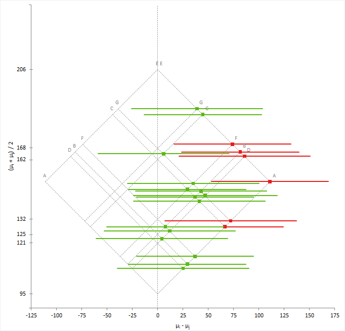
The mean-mean scatter plot shows the mean of a group on the horizontal axis against the mean of the other group on the vertical axis with a dot at the intersection. A vector centered at the intersection with a slope of -1 and a length proportional to the width of the confidence interval represents the confidence interval. A gray identity line represents equality of means; that is the difference is equal to zero. If the vector does not cross the identity line, you can conclude there is a significant difference between the means.

To make interpretation easier, a 45-degree rotated version of the plot shows the difference between means and its confidence interval on the horizontal axis against average of the means on the vertical axis.

Methods of controlling the Type I error and dependencies between parameters when making multiple comparisons between many means/medians of independent samples.

Compare the means/medians of many independent samples.

1. Select a cell in the dataset.
2. On the Analyse-it ribbon tab, in the Statistical Analyses group, click Compare Groups, and then click the multiple comparisons procedure.
   The analysis task pane opens.
3. In the Y drop-down list, select the quantitative response variable.
4. In the X drop-down list, select the categorical factor variable identifying the groups.
5. In the Type drop-down list, select the comparisons, and then:
   • If comparing with best, in the Best drop-down list, select the "best" group.
   • If comparing against a control, in the Control drop-down list, select the control group.
6. Optional: To sort the contrasts by the magnitude of the difference, select the Ordered check box.
7. Optional: In the Method drop-down list, select the multiple comparisons procedure, and in the Confidence interval edit box, type the confidence level as a percentage, or type - to suppress the confidence interval, and then in the Confidence bounds drop-down list, select the limits.
8. Optional: To perform a hypothesis test to test if the difference is equal to 0, select the Hypothesis test check box, and then to compare the p-value, in the Significance level edit box, type the predefined significance level.
9. Optional: To show a mean-mean scatter plot, select the Mean-Mean scatter plot check box.
10. Click Calculate.

A homogeneity hypothesis test formally tests if the populations have equal variances.

Many statistical hypothesis tests and estimators of effect size assume that the variances of the populations are equal. This assumption allows the variances of each group to be pooled together to provide a better estimate of the population variance. A better estimate of the variance increases the statistical power of the test meaning you can use a smaller sample size to detect the same difference, or detect smaller differences and make sharper inferences with the same sample size.

When the test p-value is small, you can reject the null hypothesis and conclude that the populations differ in variance.

Tests for the homogeneity of variance of independent samples and their properties and assumptions.

Test if the variances of two or more independent samples are equal.

1. Select a cell in the dataset.
2. On the Analyse-it ribbon tab, in the Statistical Analyses group, click Compare Groups, and then click the hypothesis test.
   The analysis task pane opens.
3. In the Y drop-down list, select the quantitative response variable.
4. In the X drop-down list, select the categorical factor variable identifying the groups.
5. In the Hypotheses drop-down list, select the null and alternative hypothesis.
6. Optional: To compare the p-value against a predefined significance level, in the Significance level edit box, type the maximum probability of rejecting the null hypothesis when in fact it is true (typically 5% or 1%).
7. Click Calculate.

Compare groups analysis study requirements and dataset layout.