Reference interval

A reference interval (sometimes called a reference range or normal range) describes the range of values of a measured quantity in healthy individuals.

• Reference limits
  A reference limit defines a value where a given proportion of reference values are less than or equal to. A reference interval defines the interval between a lower and upper reference limit that includes a given proportion of the reference values.
• Histogram
  A histogram shows the distribution of the data to assess the central tendency, variability, and shape.
• Box plot
  A box plot shows the five-number summary of the data – the minimum, first quartile, median, third quartile, and maximum. An outlier box plot is a variation of the skeletal box plot that also identifies possible outliers.
• Normal probability (Q-Q) plot
  A normal probability plot, or more specifically a quantile-quantile (Q-Q) plot, shows the distribution of the data against the expected normal distribution.

A reference limit defines a value where a given proportion of reference values are less than or equal to. A reference interval defines the interval between a lower and upper reference limit that includes a given proportion of the reference values.

The process of defining a reference interval is that reference individuals compromise a reference population from which is selected a reference sample group on which are determined reference values on which is observed a reference distribution from which are calculated reference limits that define a reference interval.

A point estimate of a reference limit is a single value that is the best estimate of the true unknown parameter; a confidence interval is a range of values and indicates the uncertainty of the estimate. It is important to remember that the width of the confidence interval is dependent upon sample size and that large sample sizes are required to produce narrow confidence intervals, particularly for skewed distributions (Linnet, 2000).

There are numerous quantile estimators that may define the reference limits. The best estimator depends heavily on the shape of the distribution.

• Normal theory quantile
  A quantile estimator derived from a normally distributed population with unknown mean and standard deviation.
• Quantile
  A distribution-free (non-parametric) quantile estimator based on the order statistics (the sorted values in the sample).
• Bootstrap quantile
  A distribution-free (non-parametric) quantile estimator that is the median of a set of quantiles calculated by re-sampling the original sample a large number of times and computing a quantile for each sample.
• Harrell-Davis quantile
  A distribution-free (non-parametric) estimator that is a weighted linear combination of order statistics. It is substantially more efficient than the traditional estimator based on one or two order statistics.
• Robust bi-weight quantile
  A quantile estimator that uses robust estimators of location and spread, which resist the effects of extreme observations.

A quantile estimator derived from a normally distributed population with unknown mean and standard deviation.

A normal theory quantile is most powerful when a random sample is from a population with a normal distribution.

In many cases, the data are skewed to the right and do not follow a normal distribution. A Box-Cox (or logarithmic) transform can correct the skewness, allowing you to use the Normal theory quantile. If not, a distribution-free estimator may be more powerful (IFCC, 1987).

A distribution-free (non-parametric) quantile estimator based on the order statistics (the sorted values in the sample).

There are several definitions for the quantile estimator useful in defining reference limits.

A 95% reference interval (0.025 and 0.975 quantiles) requires a minimum sample size of 39. A 90% confidence interval for a 95% reference interval requires a minimum sample size of 119.

A distribution-free (non-parametric) quantile estimator that is the median of a set of quantiles calculated by re-sampling the original sample a large number of times and computing a quantile for each sample.

The bootstrap quantile (Linnet, 2000)as providing the lowest root-mean-squared-error (an estimate of the bias and precision in the estimate) for both normal and skewed distributions. Another advantage is that confidence intervals can be computed for smaller sample sizes, although Linnet still recommends a sample size of at least 100.

A distribution-free (non-parametric) estimator that is a weighted linear combination of order statistics. It is substantially more efficient than the traditional estimator based on one or two order statistics.

A quantile estimator that uses robust estimators of location and spread, which resist the effects of extreme observations.

The robust bi-weight estimator (Horn & Pesce 1998) uses robust estimators of location and spread, which resist the effects of extreme observations. It requires a symmetric distribution. If the distribution is skewed, you should apply a transform to achieve symmetry, or create a new sample by mirroring the sample around the median to form a symmetric distribution (Horn, 1990), before applying the bi-weight estimator.

Estimate the reference limit or reference interval using a quantile estimator.

1. Select a cell in the dataset.
2. On the Analyse-it ribbon tab, in the Statistical Analyses group, click Diagnostic, and then under the Reference Interval heading, click the estimator.
   The analysis task pane opens.
3. In the Y drop-down list, select the variable.
4. In the Type drop-down list, select:

   Option	Description
   Reference interval	Estimate lower and upper reference limits that a stated proportion of values are between.
   Reference limit	Estimate a single reference limit that a stated proportion of values are less than.

5. In the Proportion inside interval/Proportion less than edit box, type the reference level as a percentage.
6. In the Method drop-down list, select the computation method.
7. In the Confidence interval edit box, type the confidence level as a percentage, or type - to suppress the confidence interval, and then in the drop-down list, select the confidence bounds.
8. Optional: To split the reference values by factors such as gender or age:
   1. On the Analyse-it ribbon tab, in the Reference Interval group, click Partition
   2. In the Factors list, select the factor variables.
   3. In the Partitions list, select a partition.

      The tasks change to the analysis options for that partition.

   4. Optional: By default, the analysis options are the same for each partition, set the specific analysis options for the partition as required.
   5. Repeat steps 8.c through 8.d for each partition.
9. Click Calculate.

A histogram shows the distribution of the data to assess the central tendency, variability, and shape.

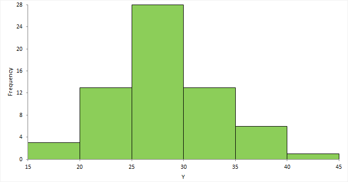
A histogram for a quantitative variable divides the range of the values into discrete classes, and then counts the number of observations falling into each class interval. The area of each bar in the histogram is proportional to the frequency in the class. When the class widths are equal, the height of the bar is also proportional to the frequency in the class.

Choosing the number of classes to use can be difficult as there is no "best," and different class widths can reveal or hide features of the data. Scott's and Freedman-Diaconis' rules provide a default starting point, though sometimes particular class intervals make sense for a particular problem.

The histogram reveals if the distribution of the data is normal, skewed (shifted to the left or right), bimodal (has more than one peak) and so on. Skewed data can sometimes be transformed to normal using a transformation. Bi-modality often indicates that there is more than one underlying population in the data. Individual bars distanced from the bulk of the data can indicate the presence of an outlier.

A box plot shows the five-number summary of the data – the minimum, first quartile, median, third quartile, and maximum. An outlier box plot is a variation of the skeletal box plot that also identifies possible outliers.

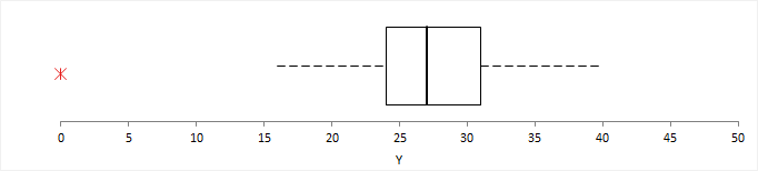
An outlier box plot is a variation of the skeletal box plot, but instead of extending to the minimum and maximum, the whiskers extend to the furthest observation within 1.5 x IQR from the quartiles. Possible near outliers (orange plus symbol) are identified as observations further than 1.5 x IQR from the quartiles, and possible far outliers (red asterisk symbol) as observations further than 3.0 x IQR from the quartiles. You should investigate each possible outlier before deciding whether to exclude it, as even in normally distributed data, an outlier box plot identifies approximately 0.7% of observations as possible outliers.

A normal probability plot, or more specifically a quantile-quantile (Q-Q) plot, shows the distribution of the data against the expected normal distribution.

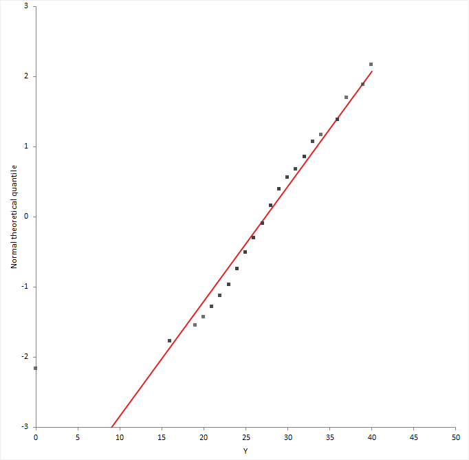
For normally distributed data, observations should lie approximately on a straight line. If the data is non-normal, the points form a curve that deviates markedly from a straight line. Possible outliers are points at the ends of the line, distanced from the bulk of the observations.

Test if a reference distribution is normal.

1. Activate the analysis report worksheet.
2. On the Analyse-it ribbon tab, in the Reference Interval group, click Normality.
   The analysis task pane Normality panel opens with the Normal plot check box selected.
3. Optional: To perform a formal normality hypothesis test, select the Normality test check box.
4. Click Recalculate.

Transform the reference values to achieve a normal distribution.

1. Activate the analysis report worksheet.
2. On the Analyse-it ribbon tab, in the Reference interval group, click Transform, and then click the transformation.
   The analysis task pane Transform panel opens.
3. Set the transform parameters:
   • If the transform is the logarithm, in the Base edit box, type the base of the logarithm or enter - for the natural logarithm.
   • If the transform is Box-Cox, in Shift and Lambda edit boxes, type the parameters, or to estimate them from the data, click Estimate unknown parameter.
   • If the transform is exponential, in the Gamma edit box, type parameter.
   • If the transform is 2-stage exponential/modulus, in the Gamma and Kappa edit boxes, type parameters.
4. Click Recalculate.

Transfer a reference limit or reference interval from one method or laboratory to another.

1. Select a cell in the dataset.
2. On the Analyse-it ribbon tab, in the Statistical Analyses group, click Diagnostic, and then under the Reference Interval heading, click Transference.
   The analysis task pane opens.
3. In the Y drop-down list, select the variable.
4. Optional: To split the reference values by factors such as gender or age:
   1. On the Analyse-it ribbon tab, in the Reference Interval group, click Partition
   2. In the Factors list, select the factor variables.
   3. In the Partitions list, select a partition.

      The tasks change to the analysis options for that partition.

   4. Optional: By default, the analysis options are the same for each partition, set the specific analysis options for the partition as required.
   5. Repeat steps 4.c through 4.d for each partition.
5. In the Reference level and Reference interval edit boxes, type the reference level as a percentage and the upper/lower reference limits.
6. Optional: If transferring from another measurement procedure, under the Linear transformation heading, in the Constant and Proportional edit boxes, type the constant and proportional average bias (available from the method comparison study) to translate the old reference limits to the new measurement procedure.
7. Select the Hypothesis test check box.
8. In the Hypotheses drop-down list, select the null and alternative hypotheses.

   The default null hypothesis is that the proportion of observations in the reference interval is equal to the reference level (95% default) against the alternative hypothesis that there are more or fewer observations in the interval. CLSI EP28-A3 performs a one-sided hypothesis test that proportion inside the interval is greater than or equal to 95% against the alternative that less than 95% are inside the interval.

9. In the Significance level edit box, type the maximum probability of rejecting the null hypothesis when in fact it is true (typically 5% or 1%).

   You need at least 20 samples for a one-sided hypothesis test at the 5% significance level. More samples are required to be able to detect a significant difference for the two-sided hypothesis test, or when a smaller significance level is required.

10. If you selected partition factors, in the Partitions list, select another partition, and then repeat steps 5 through 9 for all partitions.
11. Click Calculate.

Reference interval study requirements and dataset layout.