Regression analysis with full diagnostics Simple, polynomial, multiple and ANCOVA regression — with leverage plots, residual diagnostics, Cook’s D influence analysis, VIF, standardised betas and prediction from the fitted model.

Every feature from all five editions for 15 days.
Standard edition from US$ 155 a year · 30-day money-back guarantee.
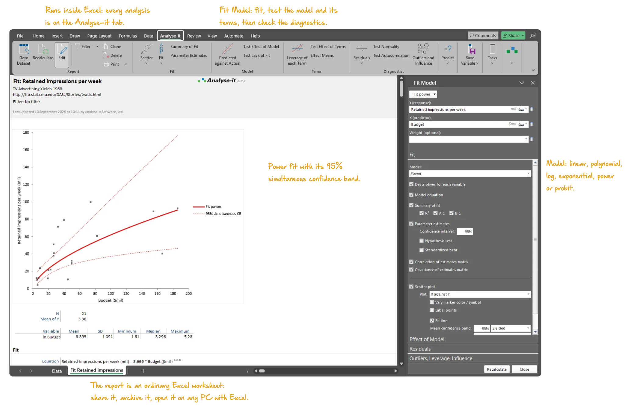
Microsoft Excel with the Analyse-it tab selected, showing a simple regression report of retained impressions per week against TV advertising budget for 21 firms: the scatter plot with the power fit line and its 95% simultaneous confidence band, N and the descriptive statistics beneath, the Fit Model and Diagnostics groups on the ribbon, and the Fit Model task pane open. Handwritten notes: Runs inside Excel: every analysis is on the Analyse-it tab; Fit Model: fit, test the model and its terms, then check the diagnostics; Power fit with its 95% simultaneous confidence band; Model: linear, polynomial, log, exponential, power or probit; The report is an ordinary Excel worksheet: share it, archive it, open it on any PC with Excel.

Regression as a process, not a single calculation

Excel’s Analysis ToolPak fits a straight line by least squares and stops. No polynomial, logarithmic or power fits without transforming the data by hand; no categorical predictors without coding the dummy variables yourself; no VIF, no leverage, no Cook’s D. A regression result is only as good as the assumptions behind it. Influential observations pull the line towards themselves. Correlated predictors inflate the standard errors until nothing looks significant. Non-constant variance makes the confidence intervals meaningless at one end of the range. The coefficients can look fine while the conclusions are wrong — and without diagnostics, you will not know.

Which model form fits the relationship? Which predictors matter, and which are redundant? Are a few unusual observations driving the result? Regression is a cycle, not a single pass from data to p-value. Fit a model, check whether the assumptions hold, find what is distorting the result, adjust and re-fit, until the model can be trusted.

Simple linear, polynomial, logarithmic, exponential, power and probit fits

The model should follow the relationship, not force a shape onto it. Fit a straight line, a polynomial up to 6th order, or a logarithmic, exponential, power or probit curve. Transform X or Y directly when a raw fit is not adequate. The scatter plot with the fit line and confidence bands shows whether the model captures the pattern or forces a shape that is not there. The F-test for lack of fit checks whether a simple model captures the relationship or the data call for a more complex form. If a linear fit shows significant lack of fit, try a polynomial or a transform before reporting a result that does not match the data.

  • Simple linear regression
  • Polynomial regression (2nd to 6th order)
  • Logarithmic regression
  • Exponential regression
  • Power regression
  • Probit regression
  • Transform X and Y variable
  • Scatter plot with fit line, confidence and prediction bands
  • Lack of fit: F-test against pure error, or χ² test against a known SD (simple models)

Multiple regression with continuous and categorical predictors

Real data have more than one predictor, and not all of them are numbers. Multiple regression takes any combination of continuous and categorical predictors, with crossed terms, polynomial terms and interactions — the same Fit Model that fits ANOVA and ANCOVA. Add categorical factors and the model reports adjusted effect means with confidence intervals for each level, with main effect and interaction plots showing how the factors combine. Five multiple comparison procedures — Tukey-Kramer, Dunnett, Hsu, Scheffé, Student’s t — test specific differences between levels, just as in ANOVA.
  • Multiple linear regression
  • Weighted regression with user-supplied weights new in v5.30
  • ANOVA
  • ANCOVA
  • Advanced models with simple, crossed, polynomial and factorial terms
  • Effect means for categorical variables
  • Main effect and interaction plots
  • Multiple comparisons of effect means
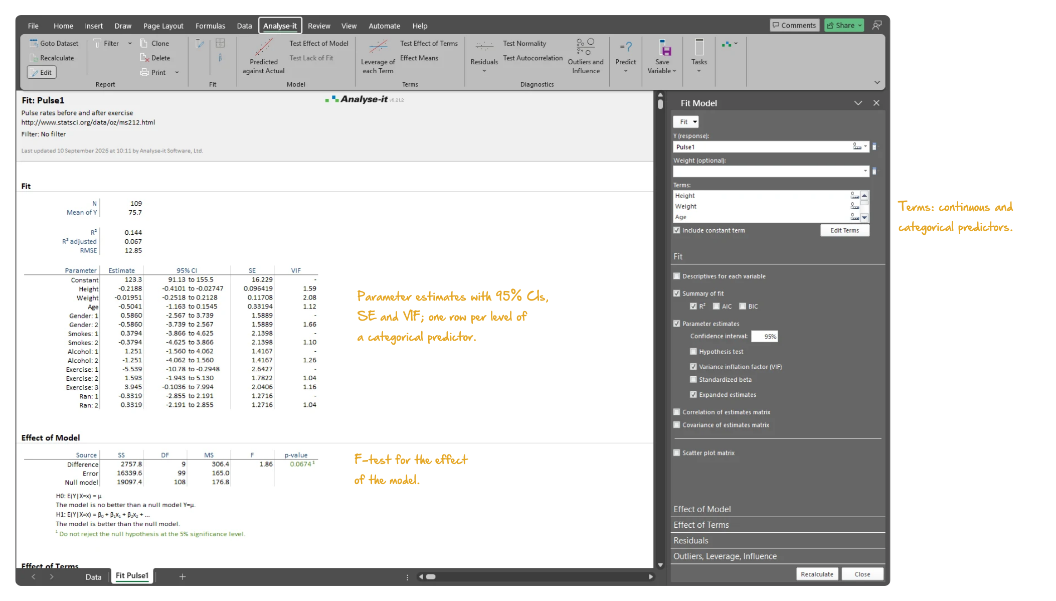
Microsoft Excel showing the Fit section of a multiple regression report of pulse rate on height, weight, age, gender, smoking, alcohol, exercise and running for 109 people: N, R-squared, adjusted R-squared and RMSE, then the parameter estimates table with a row for each level of the categorical predictors, 95% confidence intervals, standard errors and VIF, with the Fit Model task pane open on the model terms. Handwritten notes: Parameter estimates with 95% CIs, SE and VIF; one row per level of a categorical predictor; F-test for the effect of the model; Terms: continuous and categorical predictors.
Pulse rate on eight predictors, three continuous and five categorical: the parameter estimates with 95% CIs, standard errors and VIF, one row per level of a categorical predictor.

Parameter estimates with CIs, VIF, standardised betas, R², AIC and BIC

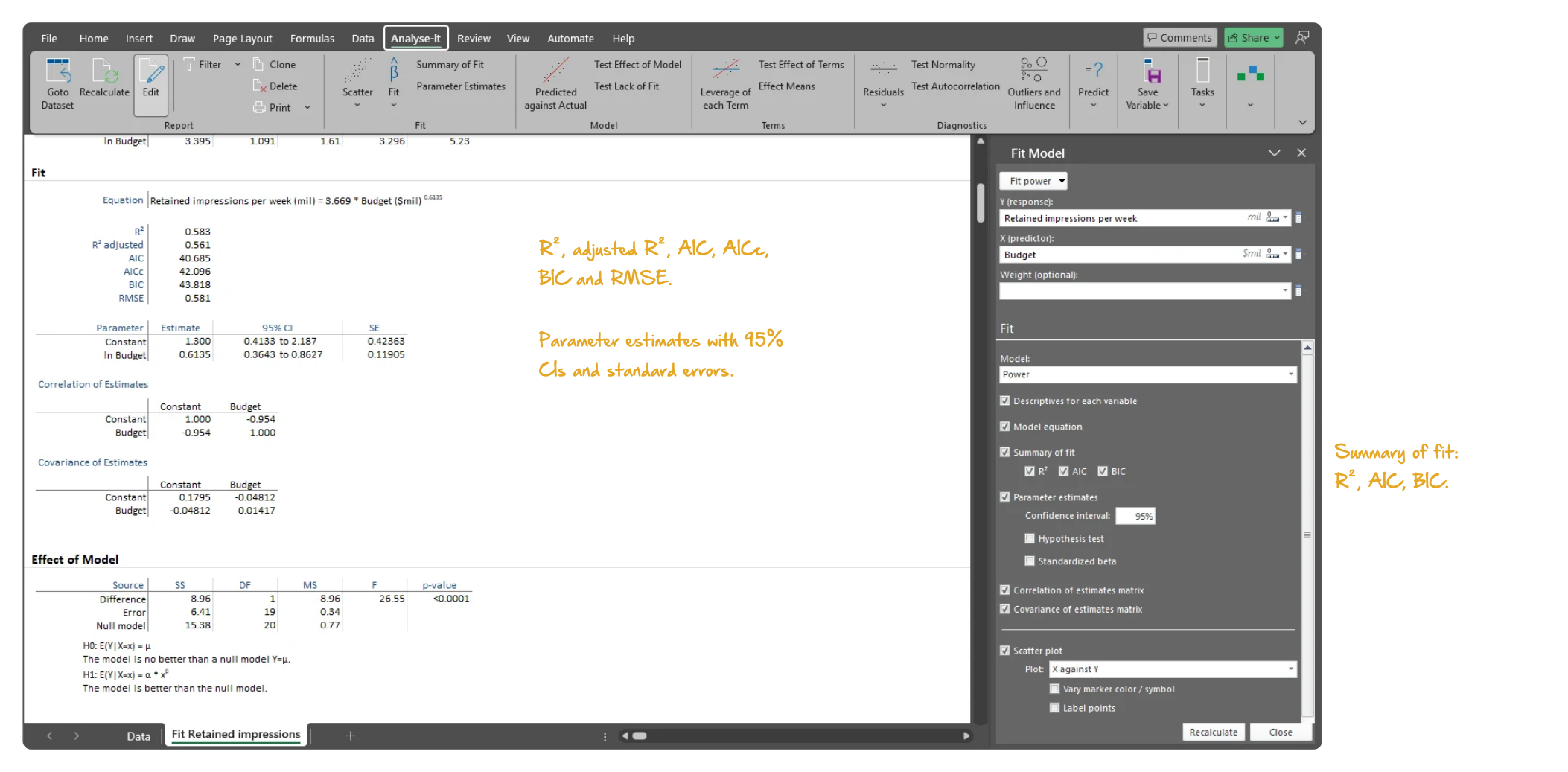
A model you cannot report and defend is not finished. Parameter estimates come with confidence intervals; VIF flags multicollinearity, and standardised betas compare the importance of predictors on a common scale. R², adjusted R², AIC and BIC compare candidate models. F-tests for the effect of the model and of each term — Type I sequential or Type III partial — show which terms matter. The model equation is there for documentation, and the predicted against actual plot shows how well the model reproduces the data.
  • Model equation
  • R², adjusted R², AIC, AICc, BIC
  • Parameter estimates with CIs, VIF, standardised betas
  • Correlation and covariance matrices of the parameter estimates
  • F-test effect of model and each term
  • Type I (sequential) and Type III (partial) tests
  • Predicted against actual plot
Microsoft Excel showing the Fit section of a simple power regression report of retained impressions on advertising budget: the model equation, R-squared 0.583, adjusted R-squared 0.561, AICc, BIC and the RMSE, the parameter estimates with 95% confidence intervals and standard errors, the correlation and covariance of the estimates, and the Effect of Model F-test beneath, with the Fit Model task pane open. Handwritten notes: R², adjusted R², AIC, AICc, BIC and RMSE; Parameter estimates with 95% CIs and standard errors; Summary of fit: R², AIC, BIC.
The power fit of retained impressions on advertising budget: model equation, R² and adjusted R², AICc, BIC, parameter estimates with 95% CIs and the Effect of Model F-test.

Leverage plots, residual plots, sequence and Lag-1 plots

Diagnostic plots show the assumption failures that the coefficients hide. A leverage plot for each term isolates that predictor’s contribution after accounting for all the others in the model. Raw and standardised residual plots reveal non-normality and heteroscedasticity; sequence and Lag-1 plots reveal autocorrelation. See the problem before it reaches the conclusion.
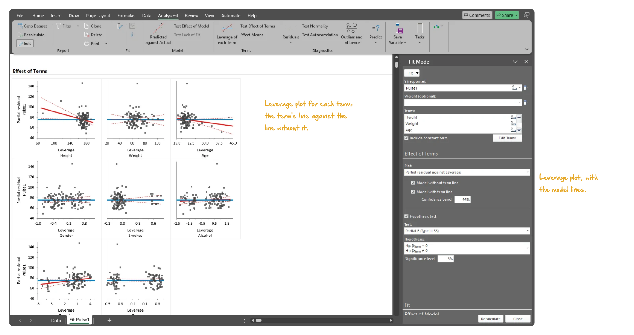
  • Leverage plot for each term
  • Residual plots (raw, standardised)
  • Sequence and Lag-1 plots
  • Durbin-Watson test for autocorrelation of residuals new in v5.30
Microsoft Excel showing the Effect of Terms section of a multiple regression report of pulse rate on eight predictors: a leverage plot for each term, height, weight, age, gender, smoking, alcohol, exercise and running, with the Fit Model task pane open on Effect of Terms. Handwritten notes: Leverage plot for each term: the term's line against the line without it; Leverage plot, with the model lines.
Leverage plots from the pulse-rate regression, one for each term in the model: each shows a predictor’s contribution after accounting for the others.

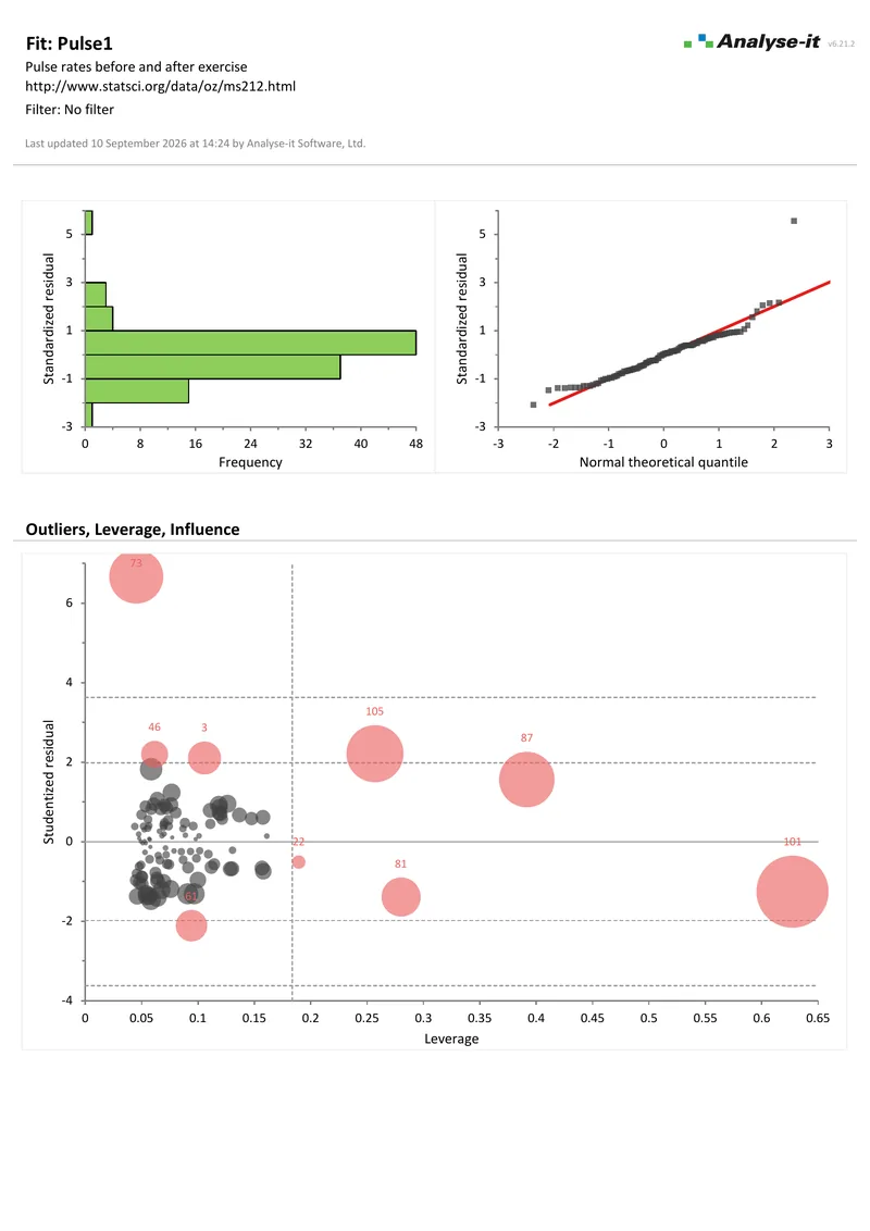
Outliers, Leverage, Influence plot: studentised residuals and Cook’s D

A few unusual cases can shift the fitted line and change the conclusion. The Outliers, Leverage, Influence plot shows the studentised residual against leverage for every observation, sized by Cook’s D. The plot shows immediately whether a few observations are distorting the model. Identify them, decide what to do about them and re-fit — the cycle of building and checking that regression needs.

  • Outliers, Leverage, Influence plot (studentised residuals against leverage, bubble size Cook’s D)
Microsoft Excel showing the Outliers, Leverage, Influence section of a multiple regression report of pulse rate on eight predictors: studentised residuals plotted against leverage for 109 observations, bubble size Cook's D, with the unusual cases labelled by observation number, and the Fit Model task pane open on the Outliers section. Handwritten notes: Studentised residual against leverage, bubble size Cook's D; influential cases labelled; Plot type, and labelling of influential cases.
Studentised residual against leverage for the 109 pulse-rate observations, bubble size Cook’s D, with the unusual cases labelled by observation number.

Predict Y for X, save fitted values, residuals, leverage and Cook’s D

The fitted model is for using, not only for reporting. Predict Y for new X values directly from the model, with no manual calculation from the coefficients. Save fitted values, residuals, standardised and studentised residuals, leverage and Cook’s D back to the dataset as new columns, ready for further investigation or reporting.

  • Predict Y for X: mean with confidence interval, individual with prediction interval
  • Inverse prediction of X for a given Y with confidence interval new in v5.90
  • Predictions and inverse predictions plotted on the scatter plot new in v5.90
  • Save fitted values, residuals, standardised residuals, studentised residuals, leverage, Cook’s D

Example analyses

See regression results in detail — parameter estimates, leverage plots, residual diagnostics and influence analysis — using real datasets you can download and follow along with.

Fit Model 1 4 pages Simple regression, power fit
TV advertising budget against retained impressions.
21 observations. Power function fit with a 95% confidence band, R², AIC, AICc and BIC, parameter estimates with CIs, correlation and covariance of the estimates, residual plot, normality diagnostics and an outlier, leverage and influence plot.
Fit Model 2 p4 4 pages Multiple regression
Pulse rates before and after exercise, 8 predictors.
109 observations, three continuous predictors and five categorical. Parameter estimates with 95% CIs and VIF, F tests for each term, leverage plots for every predictor, residual diagnostics and an outlier, leverage and influence plot.
Fit Model 3 2 pages Binary logistic regression
Intensive care unit survival, 17 predictors.
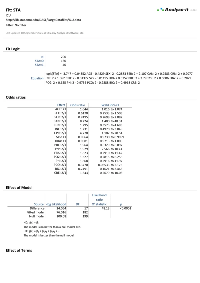
200 observations. Odds ratios with Wald 95% CIs and likelihood ratio tests for the model and for each term. Age, cancer, CPR, systolic blood pressure and admission type are significant at 5%.

Part of the Standard edition

Regression is one part of a complete statistical analysis toolkit. The Standard edition also includes ANOVA and ANCOVA, logistic regression, PCA and factor analysis, descriptive statistics, hypothesis testing, correlation and categorical data analysis. See everything in the Standard edition →

Related guides in the Learn section: fitting a calibration curve, why correlation is the wrong statistic for method comparison and choosing a regression for method comparison.

Software you can trust

Validated calculations Every statistic tested against the NIST Statistical Reference Datasets, published datasets and thousands of internal test cases. No reliance on Excel’s built-in functions. How Analyse-it is developed and validated →
Data stays on your PC No cloud processing, no uploads, no third-party access. Your data never leaves your computer — essential when working with sensitive, confidential or patient-identifiable data.
Standard Excel workbooks Analyses are ordinary Excel workbooks that you can share with colleagues, archive for audit and open on any machine with Excel — no Analyse-it licence required.
No formulas to break Results contain no formulas, so there is nothing to overwrite and no cell reference to break. The results you reported will be exactly what you find when you reopen the workbook.

Free trial and pricing

Try it on your own data first. The 15-day trial is every feature from all five editions — install it and start straight away.

Standard edition: US$ 155 per year or US$ 395 for a perpetual licence. Every purchase carries a 30-day money-back guarantee. Need a quote for purchasing? Add the licence to the cart and save it as a PDF quote.