Precision analysis software for method validation Variance component analysis with flexible nested designs — repeatability, intermediate precision and precision profiles across the measuring range. Designs cover the EP05-A3 and EP15-A3 studies, and any nesting your own experiment needs.

Every feature from all five editions for 15 days.
Method Validation edition from US$ 475 a year · 30-day money-back guarantee.
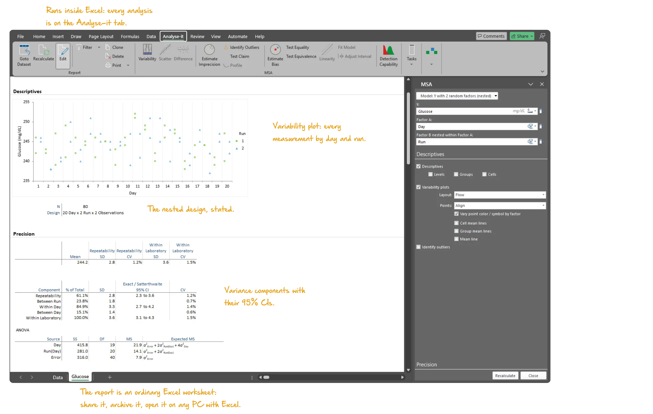
Microsoft Excel with the Analyse-it tab selected, showing the precision report for the CLSI EP05 Appendix B glucose study: the variability of measurements plot of glucose by day with the two runs coloured, N 80 and the 20 day x 2 run x 2 observation design beneath, the repeatability and within-laboratory SD and CV, the variance components table, and the Precision task pane open. Handwritten notes: Runs inside Excel: every analysis is on the Analyse-it tab; Variability plot: every measurement by day and run; The nested design, stated; Variance components with their 95% CIs; The report is an ordinary Excel worksheet: share it, archive it, open it on any PC with Excel.

Separate the sources of variability in your measurement procedure

I used Analyse-it for many product development, product troubleshooting, and technology evaluation activities... your product was the easiest to use, was accurate, and produced publication ready reports.
Stanley F. Cernosek, Ph.D.
Clinical Chemistry Reagent Development
Beckman Coulter, Inc.

Excel’s STDEV function returns one standard deviation for the whole dataset and stops. No separation of repeatability from between-run and between-day variation, no confidence interval on the estimate, no precision profile across the measuring range. Knowing the total imprecision is not enough. A method with a high overall CV might have excellent within-run repeatability but large between-day drift — a different problem from one that is noisy within every run.

Which source of variability dominates? Does the imprecision rise at low concentrations, or stay constant across the range? Does the observed precision meet the manufacturer’s claim? Without separating the variance components you cannot take targeted corrective action, and you cannot produce the precision data that regulatory submissions and accreditation inspections require.

Nested designs with up to three random factors and one fixed factor

The experiment design should match the way your laboratory operates, not the reverse. Up to three random nested factors — days, runs, operators, sites, lots — plus one fixed factor for concentration level, in any arrangement, balanced or unbalanced. The designs cover the EP05-A3 and EP15-A3 studies and any nesting your own experiment needs. Run 3 sites × 5 days × 2 runs × 3 replicates for an IVD development study, or a simpler 20 × 2 × 2 single-laboratory design.
  • Up to 3 random nested factors
  • 1 fixed factor (e.g. level)
  • Balanced and unbalanced designs
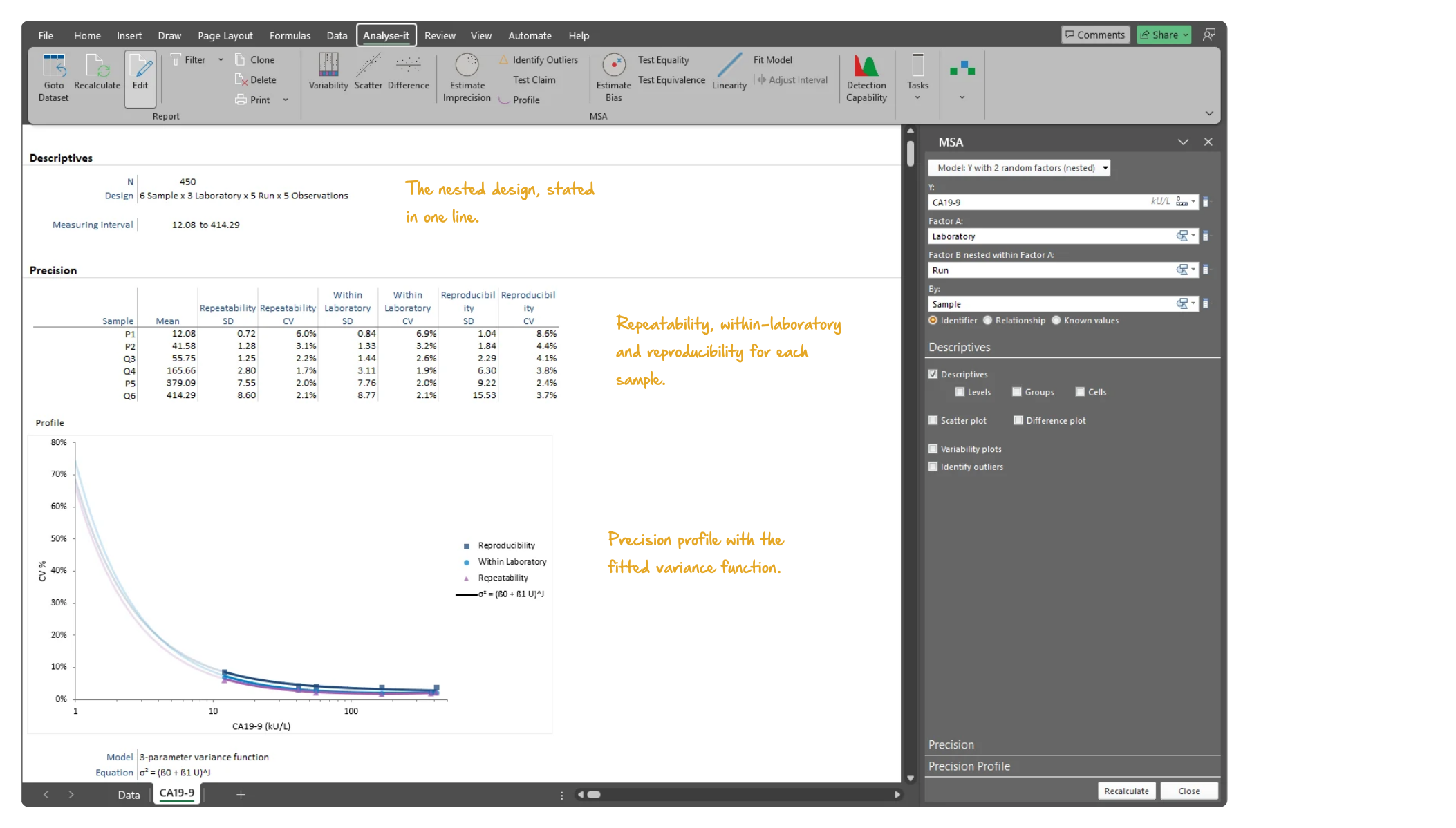
Microsoft Excel showing the precision report for the CLSI EP05-A3 Appendix B CA19-9 multi-site study: N 450, the 6 sample x 3 laboratory x 5 run x 5 observation design and the measuring interval, then the Precision summary table with the mean, repeatability, within-laboratory and reproducibility SD and CV for each of the six samples, with the Precision task pane open. Handwritten notes: The nested design, stated in one line; Repeatability, within-laboratory and reproducibility for each sample; Precision profile with the fitted variance function.
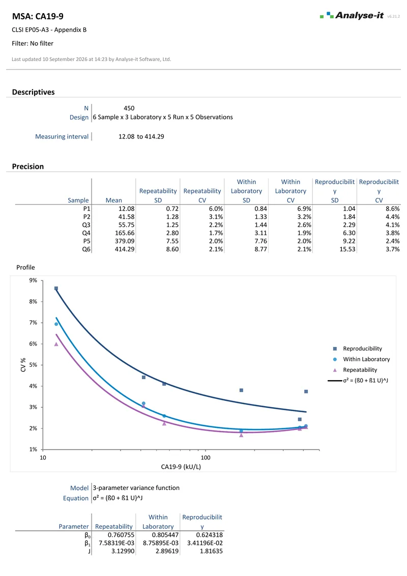
The CA19-9 multi-site study from EP05-A3 Appendix B: 6 samples × 3 laboratories × 5 runs × 5 observations. The table gives the repeatability, within-laboratory and reproducibility SD and CV of each sample.

Variance components: repeatability, within-laboratory and reproducibility

Total imprecision alone does not say where the variability comes from. Each source is reported as its own variance component, with the ANOVA table behind them: repeatability, between-run, between-day, between-operator, between-site, within-laboratory and reproducibility. Precision is expressed as variance, SD or CV% with exact, Satterthwaite and modified large-sample (MLS) confidence intervals. The terminology follows the study: total/within, reproducibility/repeatability or laboratory/repeatability.
  • Abbreviated reproducibility/repeatability and detailed intermediate precision components
  • Precision as variance, SD or CV%
  • Exact, Satterthwaite and MLS confidence intervals
  • ANOVA table
  • Total/within, reproducibility/repeatability or laboratory/repeatability
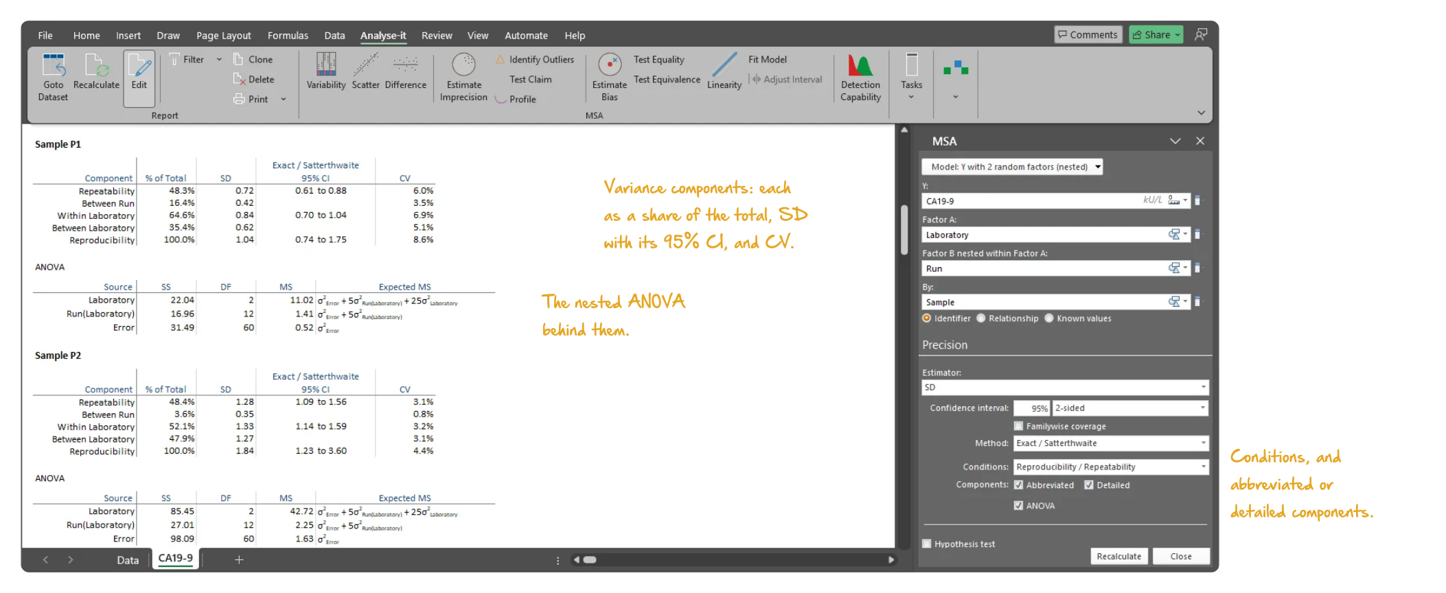
Microsoft Excel showing the Sample P1 section of the CA19-9 precision report: the variance components table with repeatability, between-run, within-laboratory, between-laboratory and reproducibility as a percentage of total, SD, 95% confidence interval and CV, and the ANOVA table with sums of squares, degrees of freedom, mean squares and expected mean squares, with the Precision task pane open. Handwritten notes: Variance components: each as a share of the total, SD with its 95% CI, and CV; The nested ANOVA behind them; Conditions, and abbreviated or detailed components.
Sample P1 of the CA19-9 study: repeatability, between-run, within-laboratory, between-laboratory and reproducibility, each as a share of the total, SD and CV with 95% confidence intervals. The ANOVA table with the expected mean squares is beneath.

Precision profiles with constant, Sadler and 4-parameter variance functions

Imprecision is rarely the same across the measuring range, and one CV at one concentration hides that. The precision profile plots SD or CV as a function of concentration with a fitted variance function. Seven models: constant variance, constant CV, mixed constant/proportional, 2-parameter linear, Sadler 3-parameter power, 3-parameter alternative power and a 4-parameter function with a turning point. The fitted variance function feeds directly into detection capability estimation (LoB, LoD, LoQ) via EP17-A2 and into total analytical error calculations.

  • SD or CV across the measuring range
  • Precision profile plot with variance function fit
  • Predict the SD or CV at any concentration from the variance function new in v5.51
  • Constant variance function
  • Constant CV function
  • Mixed constant/proportional variance function
  • 2-parameter (linear) variance function
  • Sadler 3-parameter power function
  • 3-parameter alternative power function
  • 4-parameter function with turning point
Microsoft Excel showing the precision profile of the CA19-9 precision report: CV % against concentration on a logarithmic axis for repeatability, within-laboratory precision and reproducibility, each with its fitted 3-parameter variance function, and the model, equation and parameter table beneath, with the Precision task pane open. Handwritten notes: Precision profile: CV against concentration, for each level of the design; The fitted variance function and its parameters; Variance function: seven models.
The CA19-9 precision profile: CV against concentration for repeatability, within-laboratory precision and reproducibility, with the fitted 3-parameter variance function and its parameters for each.

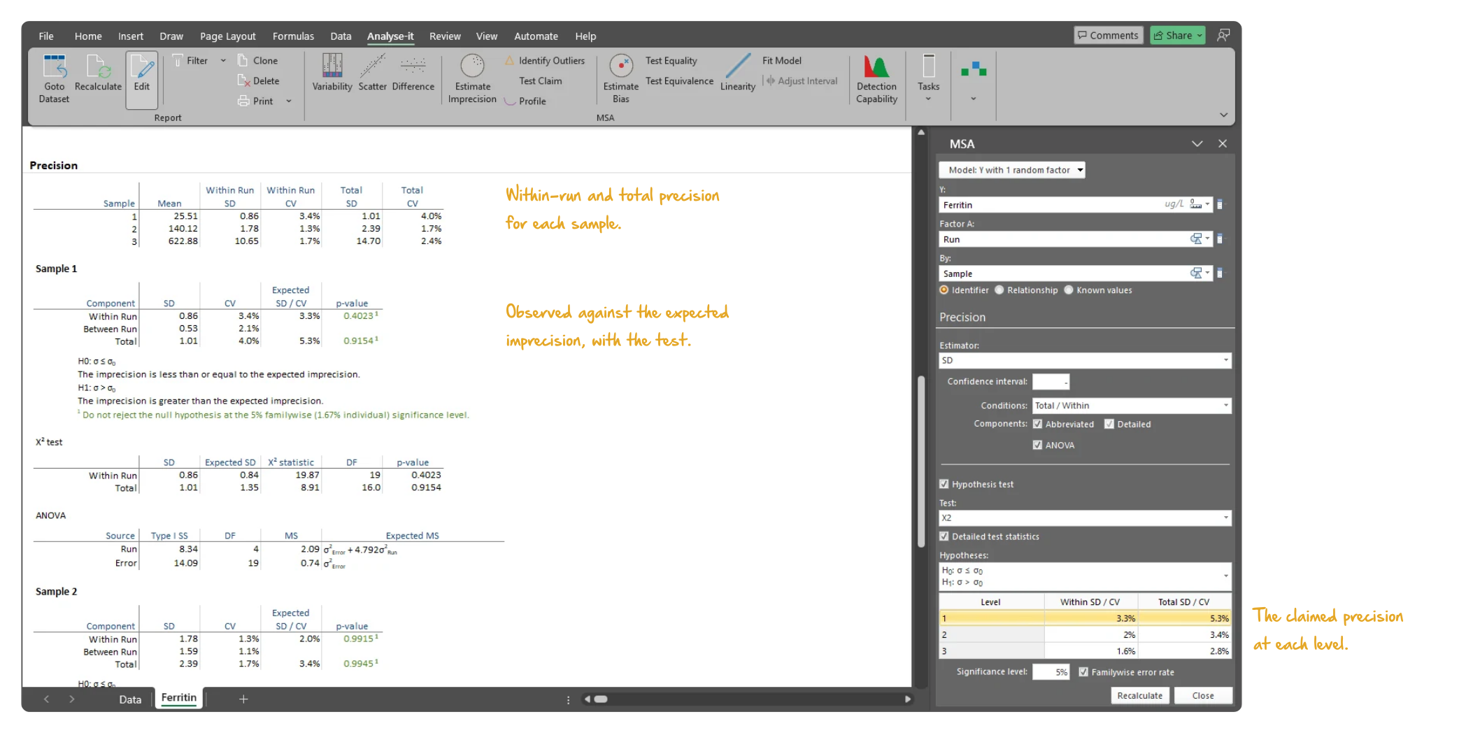
Chi-squared test of observed precision against a claim

A verification needs a pass or a fail, not a number to interpret. Test the observed precision against a precision goal — such as the manufacturer’s claimed CV of 3.5% — with the chi-squared test. The result is a formal pass/fail assessment per EP15-A3.
  • χ² test against precision claim
Microsoft Excel showing the Precision section of a ferritin precision verification report from CLSI EP15-A3: the observed precision of each sample and the chi-squared test of the observed precision against the manufacturer’s claimed imprecision, with the Precision task pane open. Handwritten notes: Within-run and total precision for each sample; Observed against the expected imprecision, with the test; The claimed precision at each level.
Ferritin verification from EP15-A3: 3 samples × 5 runs × 5 observations, with the observed precision tested against the manufacturer’s claimed imprecision.

Generalised ESD outliers and the variability of measurements plot

An aberrant result inflates the variance components, so find it before it enters the analysis. The generalised ESD test extends Grubbs’s test to multiple outliers. The variability of measurements plot shows every observation by day and run, for visual inspection of drift, shifts or individual aberrations across the dataset.

  • Generalised ESD outlier identification
  • Variability of measurements plot
  • Scatter plot
  • Difference plot

Example analyses

See precision study results in detail — variance components, ANOVA tables, precision profiles and verification tests — using CLSI example datasets you can download and follow along with.

EP05 A3 Example 1 1 page EP05-A2 — Appendix B
Glucose precision, single site.
20 days × 2 runs × 2 observations, 80 results. Variability plot, then repeatability, between-run, within-day, between-day and within-laboratory components with CIs and the ANOVA table with expected mean squares.
EP05 A3 Example 2 3 pages EP05-A3 — Appendix B
CA19-9 precision, multi-site.
6 samples × 3 laboratories × 5 runs × 5 observations, 450 results. Repeatability, within-laboratory and reproducibility for each sample, then a precision profile fitted with a three-parameter variance function.

Part of measurement system analysis

Precision is one part of measurement system analysis, alongside linearity (EP06-Ed2), bias/trueness verification (EP15-A3), preliminary evaluation (EP10-A3-AMD) and detection capability (EP17-A2). Precision profiles from EP05-A3 feed directly into detection capability estimation.

Related guides in the Learn section: establishing precision, the precision components, verifying a manufacturer’s claims and trueness, precision and accuracy. Further guides cover top-down measurement uncertainty, allowable total error and performance specifications, what CLIA requires before you report a result and performance studies for an IVD 510(k).

Software you can trust

Validated calculations you can defend at inspection Every calculation is performed by Analyse-it — no Excel formulas, no third-party functions. Results are validated against CLSI reference datasets, published datasets and thousands of internal test cases before every release. How Analyse-it is developed and validated →
Data stays in your facility Analyse-it runs entirely within Microsoft Excel on your PC. No cloud processing, no data transmission. Pre-submission data, data derived from patients and in-process results stay within your facility under your own data governance controls.
Standard Excel workbooks anyone can open Every analysis is an ordinary .xlsx workbook. Share with colleagues, submit to regulatory affairs, archive for audit, open on any PC with Excel. No proprietary format, no licence required to view results. Colleagues and auditors see exactly what you see.
Results that cannot be accidentally broken Analysis output contains computed values, not formulas. Nothing to accidentally overwrite, no cell references to break, no formula errors to introduce. The results you reported are exactly what you will find when you reopen the workbook months or years later for an audit.

Free trial and pricing

Try it on your own data first. The 15-day trial is every feature from all five editions — install it and start straight away.

Method Validation edition: US$ 475 per year or US$ 1155 for a perpetual licence. Every purchase carries a 30-day money-back guarantee. Need a quote for purchasing? Add the licence to the cart and save it as a PDF quote.