Reference interval software for method validation Establish, partition, verify, and transfer reference intervals — parametric, non-parametric, robust, bootstrap, and Harrell-Davis quantile methods with a full range of transformations. More quantile methods than EP28-A3C requires, for clinical and research reference data alike.

Every feature from all five editions for 15 days, no sign-up.
Method Validation edition from US$ 475 a year · 30-day money-back guarantee.
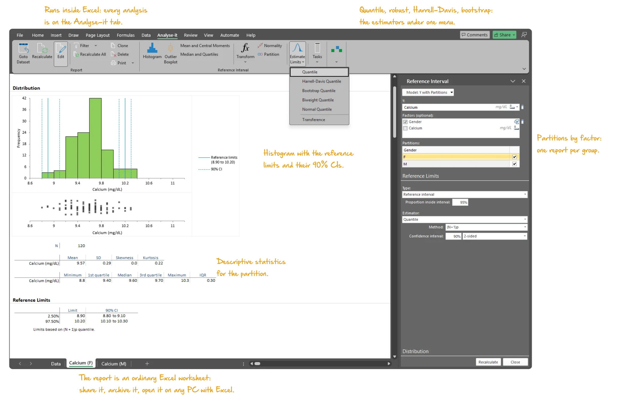
Microsoft Excel with the Analyse-it tab selected, showing a reference interval report for calcium in females: the frequency histogram with the reference limits and their 90% confidence intervals, the dot plot, descriptive statistics, the Reference Limits table, the Estimate Limits menu open on the ribbon listing the quantile, Harrell-Davis, bootstrap, biweight and normal estimators, and the Reference Interval task pane open on Reference Limits. Handwritten notes: Runs inside Excel: every analysis is on the Analyse-it tab; Quantile, robust, Harrell-Davis, bootstrap: the estimators under one menu; Histogram with the reference limits and their 90% CIs; Descriptive statistics for the partition; Partitions by factor: one report per group; The report is an ordinary Excel worksheet: share it, archive it, open it on any PC with Excel.

Establish reference ranges that reflect real patient populations

We use Analyse-it for the analysis of data necessary to file 510k. We chose Analyse-it because it works in Excel, includes CLSI protocols, and, unlike EP-Evaluator, lets us analyze data directly from equipment without typing.
Thomas D Harrigan, Ph.D.
Technical Product Manager
Alfa Wassermann Diagnostic Technologies

Excel’s PERCENTILE function returns a quantile and stops. No confidence interval on the limit, no choice of quantile method for the sample size, no transformation for skewed data, no partitioning by sex or age. Clinicians interpret every result against the reference interval. If the interval does not represent the population being tested, patients are flagged as abnormal when they are not, or genuinely abnormal results slip through.

Which quantile method suits this sample size and distribution? Should the data be transformed, or the interval partitioned by sex and age? Does an interval transferred from another measurement procedure still hold? IVD manufacturers need the answers for product labelling; clinical laboratories need them for every analyte they report.

Parametric, non-parametric, robust, bootstrap and Harrell-Davis quantiles

The quantile method should suit the sample size and the shape of the data, not the other way round. Parametric, non-parametric with three computation approaches — (N+1)p, Np+½ and (N+⅓)p+⅓ — robust bi-weight, bootstrap and Harrell-Davis, with confidence intervals on every reference limit. Run two methods on the same dataset to see how sensitive the limits are to the estimation approach. The frequency histogram shows the limits against the data.
  • Normal (parametric) quantile, Z (MVUE) or t-based
  • Non-parametric quantile: (N+1)p, Np+½, (N+1/3)p+1/3
  • Harrell-Davis quantile
  • Bootstrap quantile
  • Robust bi-weight quantile
  • Confidence intervals on all reference limits
  • Two-sided reference interval or one-sided reference limit
  • Frequency distribution histogram with normal overlay and reference limits
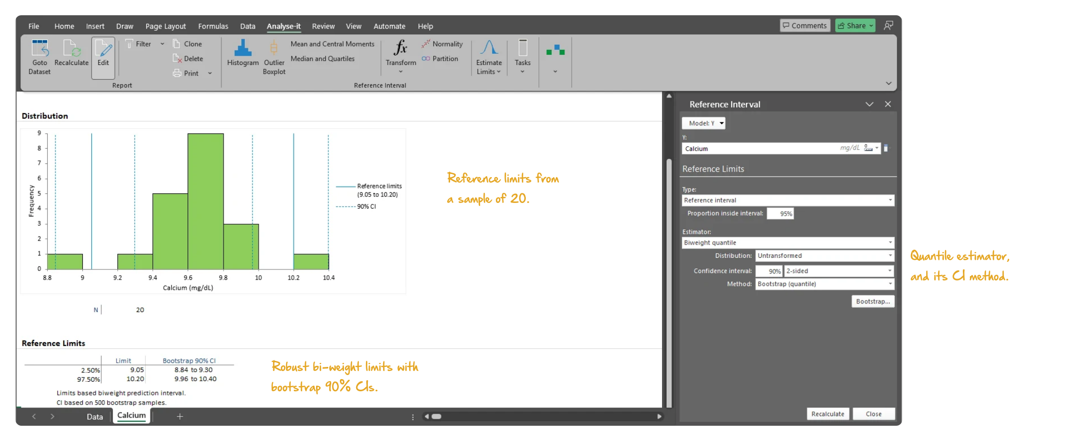
Microsoft Excel showing a reference interval report for a 20-sample calcium set: the histogram with robust bi-weight reference limits, and the Reference Limits table with bootstrap 90% confidence intervals, with the task pane open on the estimator options. Handwritten notes: Reference limits from a sample of 20; Robust bi-weight limits with bootstrap 90% CIs; Quantile estimator, and its CI method.
Robust bi-weight reference limits for a 20-observation calcium sample, with a bootstrap 90% confidence interval on each limit and the histogram above.

Partition by sex, age group, ethnicity or any combination of factors

Where a reference interval differs between subgroups, one interval for everyone misclassifies both. Partition by any combination of factors within a single analysis — sex and age group for an analyte like alkaline phosphatase, where both matter. Each subgroup keeps its own sample, its own outlier screening and its own reference limits.

  • Partition by factor(s)

Log, Box-Cox, Manly exponential and two-stage modulus transformations

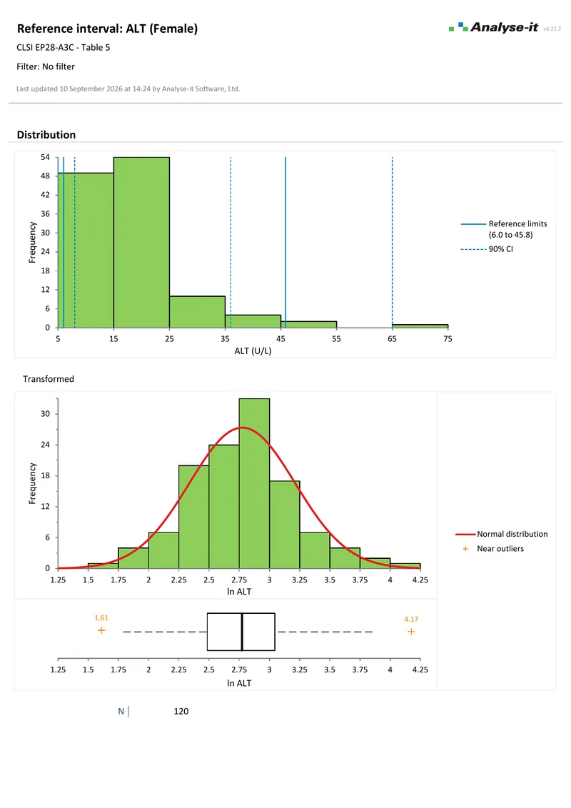
Non-normal data forced through a parametric calculation gives limits that do not fit the population. Seven transformations bring skewed data closer to normal before the limits are calculated: log, square root, cube root, reciprocal, Box-Cox, Manly exponential and two-stage exponential/modulus. The reference limits are reported back on the original measurement scale.

  • Log transformation
  • Square and cube root
  • Reciprocal transformation
  • Box-Cox
  • Manly exponential
  • 2-stage exponential / modulus
Microsoft Excel showing a reference interval report for ALT in females: the raw histogram with its reference limits, and beneath it the Transformed histogram of ln ALT with a normal curve overlaid, with the task pane open on the Transform section. Handwritten notes: Raw ALT: skewed, with its reference limits; The same data after a log transform, normal curve overlaid; Transform: log, Box-Cox, Manly or two-stage modulus.
ALT in females: the raw distribution with its reference limits, and the same data after a natural log transformation with the normal curve overlaid.

Tukey outlier box plot, Shapiro-Wilk, Anderson-Darling and normal Q-Q plot

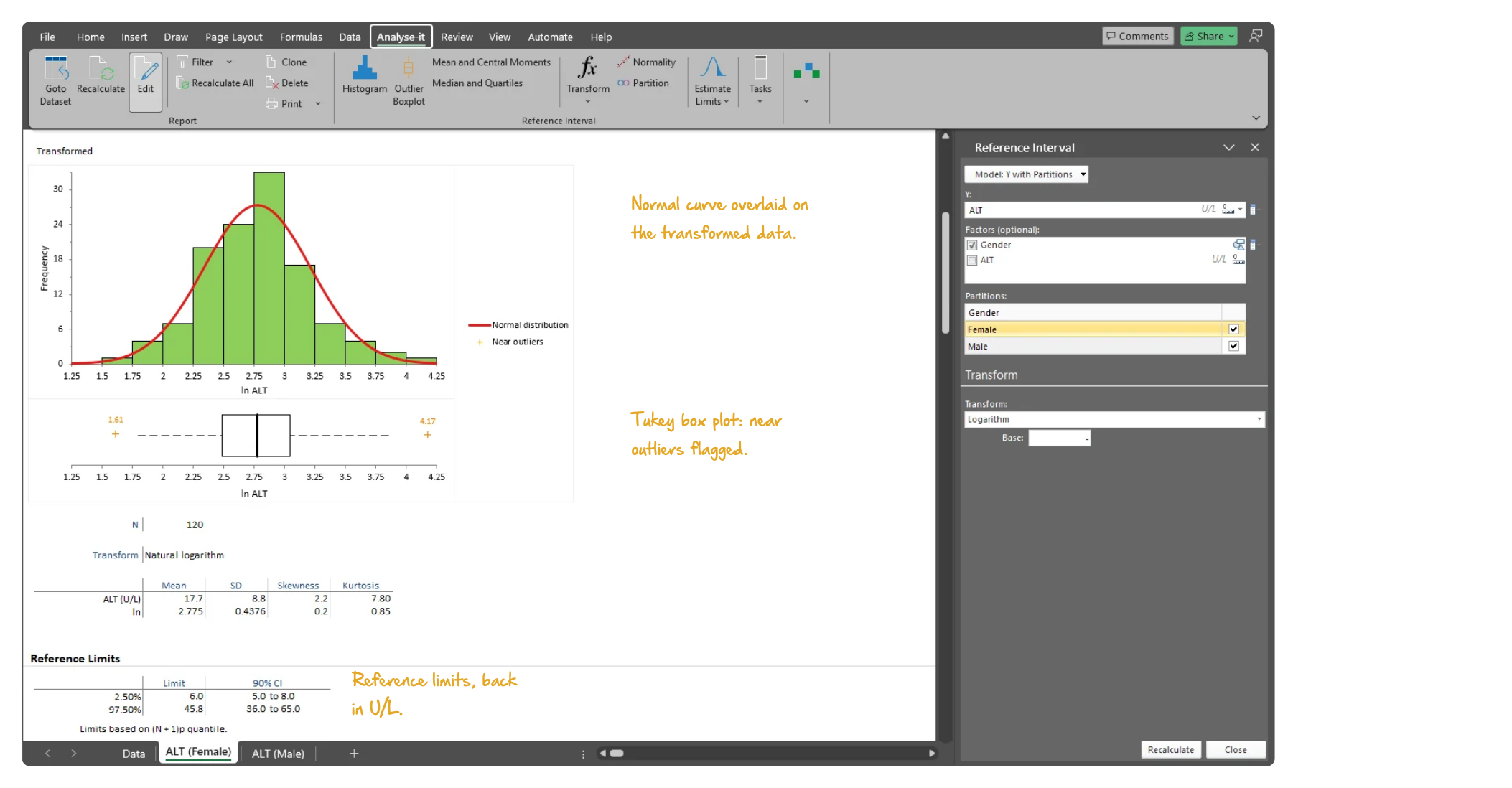
An extreme value or a wrong assumption about the distribution distorts the reference limits. The Tukey outlier box plot identifies and flags extreme values before they enter the calculation. Shapiro-Wilk and Anderson-Darling tests and a normal Q-Q plot with Lilliefors confidence band check normality, before and after transformation.
  • Tukey outlier box plot
  • Shapiro-Wilk test
  • Anderson-Darling test
  • Normal Q-Q plot with Lilliefors confidence band
Microsoft Excel showing the Transformed section of a reference interval report: the ln ALT histogram with a normal curve, the Tukey outlier box plot beneath it with near outliers marked, descriptive statistics and the Reference Limits table in U/L. Handwritten notes: Normal curve overlaid on the transformed data; Tukey box plot: near outliers flagged; Reference limits, back in U/L.
The log-transformed ALT data with the normal curve overlaid, and the Tukey outlier box plot beneath it flagging the near outliers.

Transfer by method comparison regression, verification by binomial test

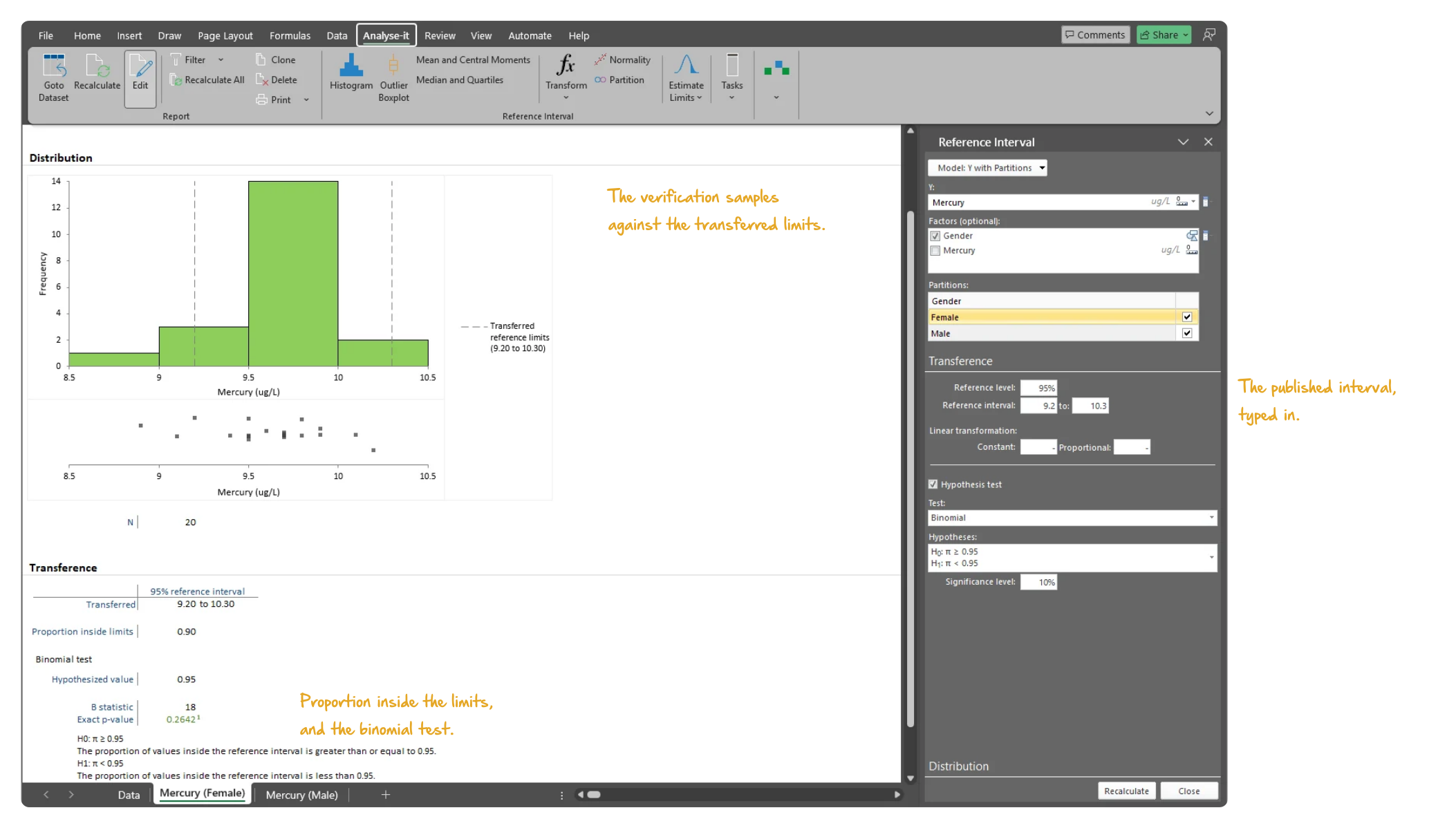
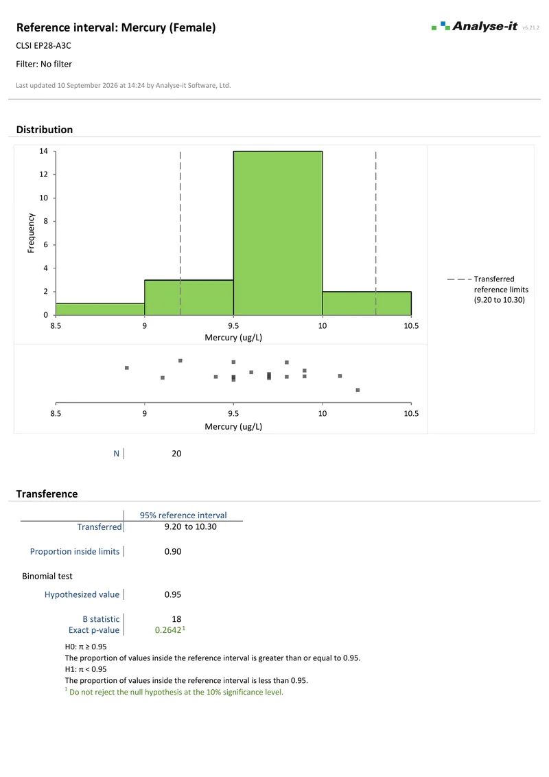
Transferring an established interval avoids recruiting a new reference population. Transfer an existing interval to a new measurement procedure using the regression function from a method comparison study. Verify the transferred limits with a binomial test for the proportion of results falling inside the interval — typically 20 samples per partition, as EP28-A3C describes.

  • Transfer using method comparison regression function
  • Binomial test for proportion inside reference interval
Microsoft Excel showing a reference interval transference report for mercury in females: the histogram of 20 verification samples with the transferred limits, the Transference table with the proportion inside the limits, and the binomial test with its p-value, task pane open on Transference. Handwritten notes: The verification samples against the transferred limits; Proportion inside the limits, and the binomial test; The published interval, typed in.
Verifying a transferred mercury reference interval: 20 samples against the transferred limits, the proportion inside them and the binomial test.

Example analyses

See reference interval results in detail — quantile methods, partitioning, transformations, and transfer/verification — using CLSI example datasets you can download and follow along with.

EP28 A3 Example 1 2 pages EP28-A3C — Table 4
Calcium reference intervals by sex.
120 observations per sex, reported separately. Distribution with descriptive statistics, and nonparametric reference limits from the (N+1)p quantile with 90% CIs.
EP28 A3 Example 2 4 pages EP28-A3C — Table 5
ALT reference intervals by sex.
120 observations per sex, both skewed. A natural log transform, then nonparametric reference limits from the (N+1)p quantile with 90% CIs on the transformed scale. Histograms on both scales, and a box plot.
EP28 A3 Example 3 2 pages EP28-A3C
Mercury reference interval transference.
20 observations per sex, tested against limits transferred from another laboratory. The proportion of results falling inside the transferred interval, with an exact binomial test against 95%.
EP28 A3 Example 4 1 page EP28-A3C — Appendix B
Calcium reference interval, robust method.
20 observations. Reference limits from the robust biweight prediction interval, with bootstrap 90% CIs from 500 samples.

Part of the Method Validation Edition

Reference intervals are one part of the Method Validation Edition, alongside measurement system analysis, method comparison, and diagnostic performance.

Related guides in our Learn section: choosing a reference interval method, transferring and verifying an interval, when to partition, handling outliers and skew, and what CLIA requires before you report a result.

Reference intervals are also in the Medical edition, with diagnostic accuracy, Bland–Altman agreement and survival analysis. For clinical and biomedical research it is the better fit, from US$ 340 a year. The Method Validation edition adds precision, linearity, detection limits and regression-based method comparison for validating a method.

Software you can trust

Validated calculations you can defend at inspection Every calculation is performed by Analyse-it — no Excel formulas, no third-party functions. Results are validated against CLSI reference datasets, published datasets, and thousands of internal test cases before every release. See how we develop and validate Analyse-it →
Data stays in your facility Analyse-it runs entirely within Microsoft Excel on your PC. No cloud processing, no data transmission. Pre-submission data, patient-adjacent data, and in-process results stay within your facility under your own data governance controls.
Standard Excel workbooks anyone can open Every analysis is an ordinary .xlsx workbook. Share with colleagues, submit to regulatory affairs, archive for audit, open on any PC with Excel. No proprietary format, no licence required to view results. Colleagues and auditors see exactly what you see.
Results that cannot be accidentally broken Analysis output contains computed values, not formulas. Nothing to accidentally overwrite, no cell references to break, no formula errors to introduce. The results you reported are exactly what you will find when you reopen the workbook months or years later for an audit.

Free trial and pricing

Try it on your own data first. The 15-day trial is every feature from all five editions, with no sign-up and no licence key — install it and start straight away.

Method Validation edition from US$ 475 per year, or US$ 1155 for a perpetual licence. Every purchase carries a 30-day money-back guarantee. Need a quote for purchasing? Add the licence to the cart and save it as a PDF quote.