Method comparison software for method validation Five regression methods and Bland-Altman in one analysis — bias at clinical decision points, replicate support, interval partitioning, and total analytical error. Deming and Passing-Bablok have been in Analyse-it since 1998, and remain available whether or not you are working to a guideline.

Every feature from all five editions for 15 days, no sign-up.
Method Validation edition from US$ 475 a year · 30-day money-back guarantee.
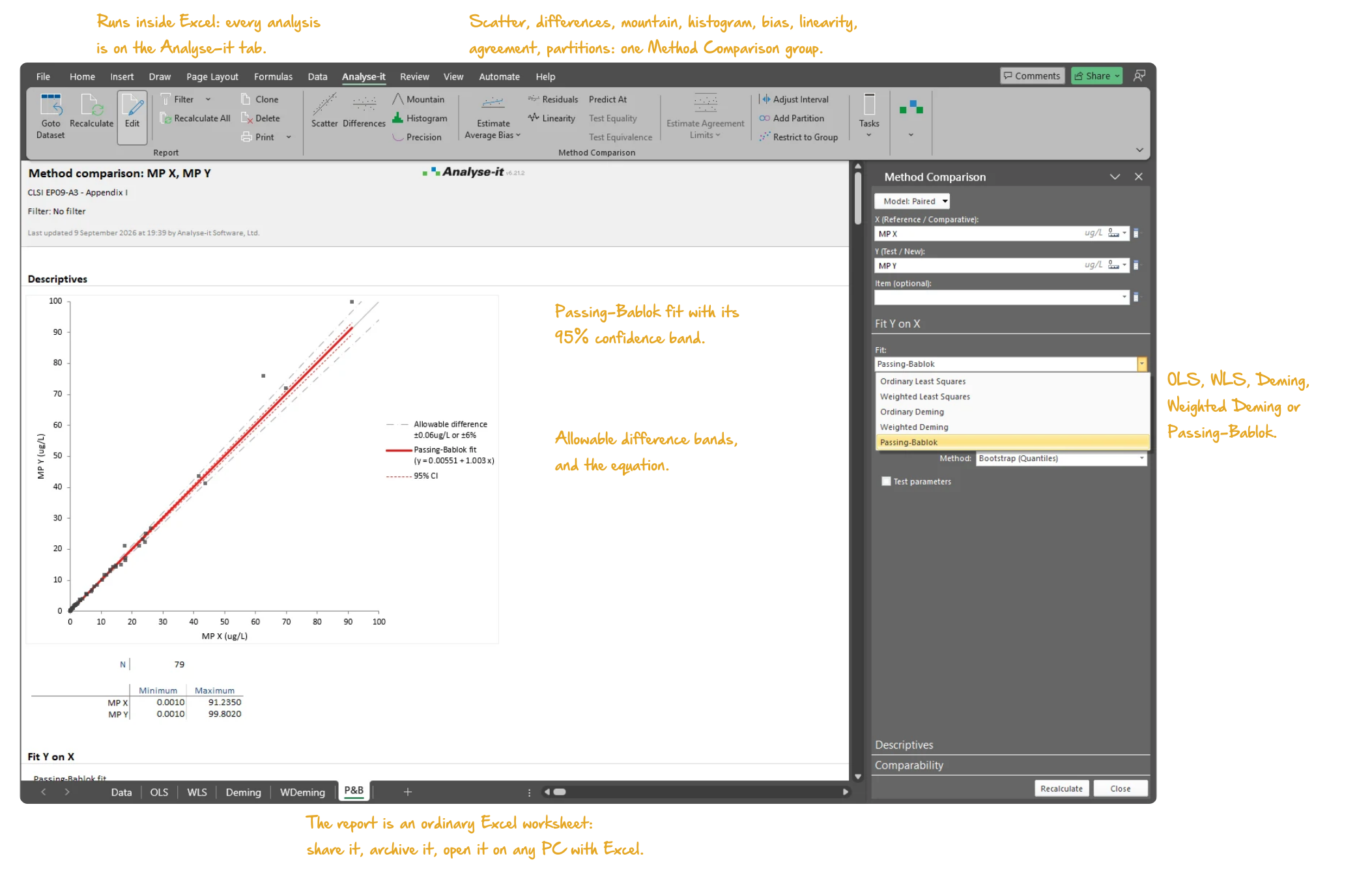
Microsoft Excel with the Analyse-it tab selected, showing a method comparison report: the scatter plot of the two methods with the Passing-Bablok fit, its 95% confidence band and the allowable difference bands, and the Method Comparison task pane open on Fit Y on X with the list of fits dropped open: ordinary least squares, weighted least squares, ordinary Deming, weighted Deming and Passing-Bablok. Handwritten notes: Runs inside Excel: every analysis is on the Analyse-it tab; Scatter, differences, mountain, histogram, bias, linearity, agreement, partitions: one Method Comparison group; Passing-Bablok fit with its 95% confidence band; Allowable difference bands, and the equation; OLS, WLS, Deming, Weighted Deming or Passing-Bablok; The report is an ordinary Excel worksheet: share it, archive it, open it on any PC with Excel.

Quantify the bias between methods and decide if it matters clinically

Excel’s LINEST function and chart trendline fit an ordinary least-squares line and stop. The reference method is assumed error-free; there is no Deming or Passing-Bablok regression, no Bland-Altman plot, no bias at a decision point. Method comparison is not a single analysis. It is a sequence of decisions, and each answer changes which regression is valid and what the bias estimate means.

Is precision constant, or does it vary across the measuring range? Are there enough samples for a non-parametric method, or is a parametric one more appropriate? Is the bias constant or proportional? Does the linear model hold? And once the bias is estimated, does it matter at the concentrations where clinical decisions are made?

Passing-Bablok, Deming, Weighted Deming, OLS and WLS regression

Which regression is valid depends on the data, so all five are available in the same analysis. Passing-Bablok, in the 1983 and extended 1988 forms, is the non-parametric starting point: robust to outliers, no distributional assumptions, no need to know the precision ratio. Deming and Weighted Deming use the known precision of both methods, constant SD or constant CV, for a more efficient estimate; OLS and WLS assume an error-free reference. Every fit reports slope and intercept with confidence intervals, systematic error split into constant and proportional bias, and Syx to flag matrix effects against expected within-run precision.
  • Passing-Bablok regression (1983 and 1988 methods)
  • Deming regression
  • Weighted Deming regression
  • Ordinary linear regression (OLS)
  • Weighted linear regression (WLS)
  • Slope and intercept with confidence intervals
  • Passing-Bablok: bootstrap and normal approximation CIs
  • Reproducible bootstrap intervals (fixed seed) new in v5.51
  • Deming/Weighted Deming: jackknife CIs
  • Systematic error: constant and proportional bias with CIs
  • Syx independent precision estimate
  • Scatter plot with fit line, confidence bands, identity line, and equation
  • Scatter plot with allowable error bands
  • Vary colour of points by a factor
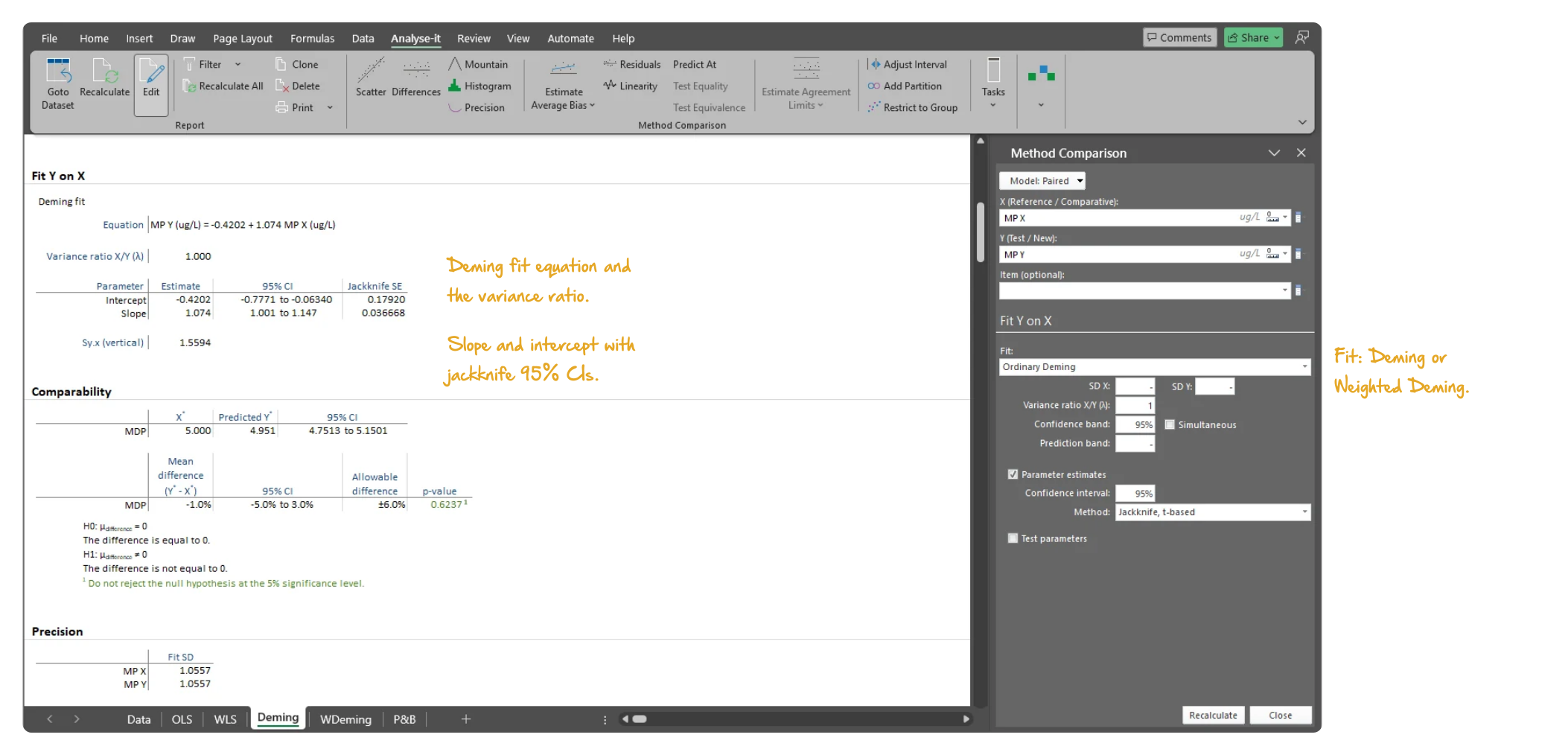
Microsoft Excel showing the Fit Y on X section of a method comparison report: the Deming fit equation, the variance ratio, and the intercept and slope with jackknife 95% confidence intervals and standard errors, then the Comparability and Precision tables, with the task pane open on the fit options. Handwritten notes: Deming fit equation and the variance ratio; Slope and intercept with jackknife 95% CIs; Fit: Deming or Weighted Deming.
Deming regression on the EP09-A3 Appendix I data: the equation, the variance ratio λ, and slope and intercept with jackknife 95% confidence intervals.

Bland-Altman limits of agreement, difference plot and mountain plot

Regression estimates the bias; the difference plot shows how the differences are distributed across the whole range. Mean, median or linear fit bias models, with constant-width limits or V-shaped limits that widen when precision is proportional to concentration. Confidence intervals on the limits themselves, not only on the bias. The mountain plot alongside shows the cumulative distribution of the differences, a second view of agreement.

  • Limits of agreement with mean, median, and linear fit bias
  • Constant and non-constant precision (horizontal and V-shaped limits)
  • Confidence intervals on the limits
  • Non-parametric (percentile) limits of agreement
  • Limits of agreement for single measurements or for the mean of replicates
  • Difference / relative difference / ratio plot against X or mean
  • Difference plot with allowable difference band and histogram
  • Linear or log X-axis on difference plots new in v5.51
  • Mountain plot with allowable difference band
Microsoft Excel showing a method comparison report for LDL cholesterol: the Bland-Altman difference plot with the 95% limits of agreement and the allowable difference band, with the task pane open on Fit Differences. Handwritten notes: Difference plot: Y - X against X; 95% limits of agreement and the allowable difference band; Bias model: mean, median or linear fit; limits.
LDL cholesterol, 100 samples, from EP21-A Table 2: the difference plot with the 95% limits of agreement and the ±10 mg/dL allowable difference band.

Bias at clinical decision points and total analytical error per EP21-A

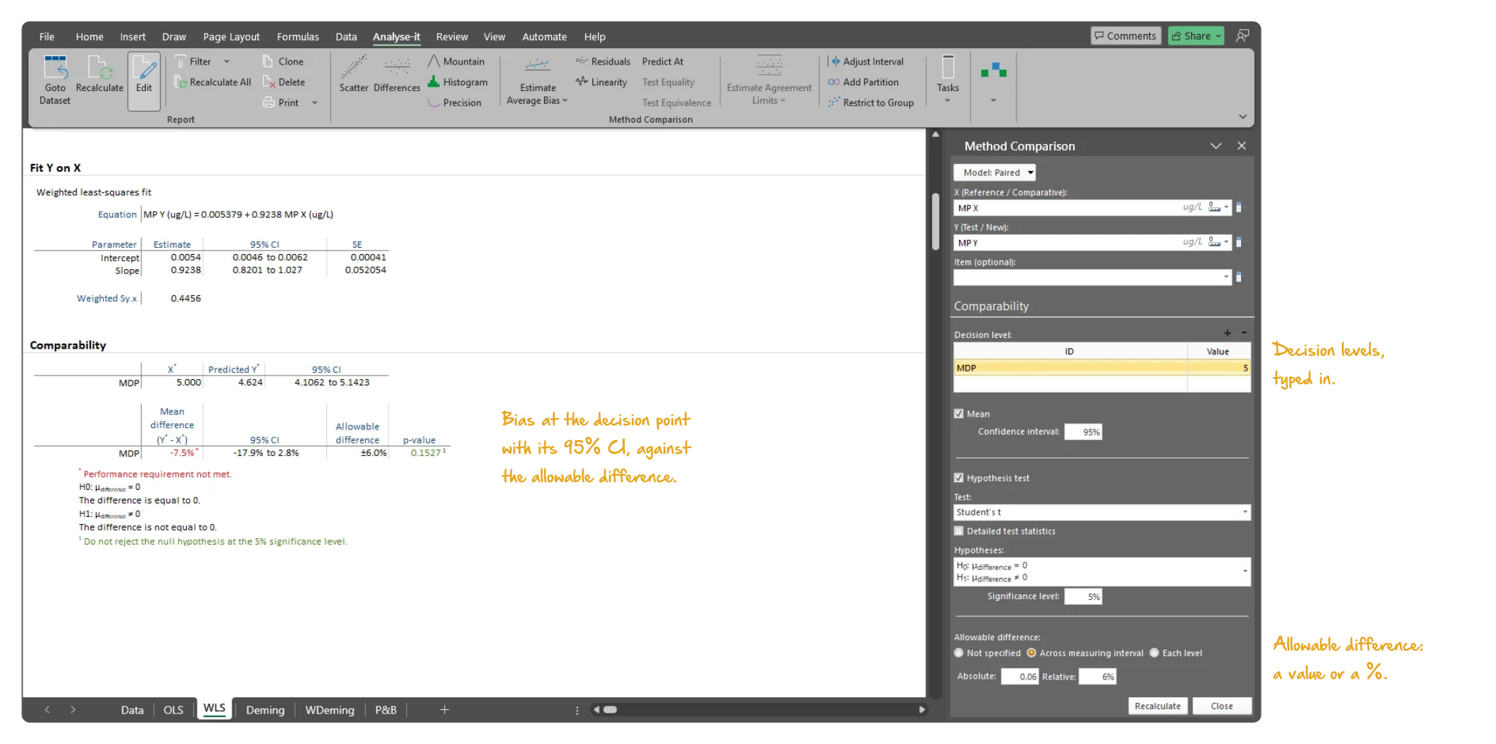
The overall slope gives the average bias, but clinical decisions happen at specific concentrations. Predict the bias, with a confidence interval, at each decision point you specify. Test equality (is there a significant difference?) and equivalence (is the difference clinically acceptable?) per EP09-A3, with the allowable difference as an absolute value, a percentage or both. A method can pass on bias and still fail when bias and imprecision together exceed the allowable total error. EP21-A adds the test method’s imprecision to the regression bias at each decision point and compares the total against allowable total error: one pass/fail assessment for both.
  • Predict bias at clinical decision points
  • Equality and equivalence tests at decision points
  • Allowable error: absolute, percentage, or combination
  • Bias + imprecision at each decision point
  • Comparison against allowable total error
  • Pass/fail assessment
Microsoft Excel showing the Comparability section of a method comparison report: the weighted least-squares fit, the predicted value at the 5 ug/L medical decision point, the mean difference with its 95% confidence interval against the allowable difference, the performance requirement footnote and the equality test, with the task pane open on Comparability. Handwritten notes: Bias at the decision point with its 95% CI, against the allowable difference; Decision levels, typed in; Allowable difference: a value or a %.
Weighted linear fit: bias at the 5 μg/L decision point with its 95% CI against the ±6% allowable difference, the equality test p-value, and the performance requirement flagged as not met.

Replicates, partitioned measuring intervals and commutability per EP14-A3

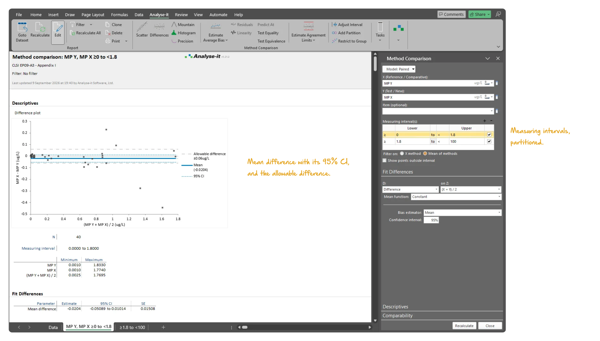
Precision that changes across the measuring range, or a material that does not behave like a patient sample, invalidates a single regression. Measure in singlicate, duplicate or replicate, with precision (SD or CV) and a precision plot for each method. Reduce the measuring interval, or partition it so each interval has its own regression, bias estimates and comparability assessment, as EP09-A3 specifies for non-constant precision. Per EP14-A3, compare each processed sample — calibrator or QC material — against the prediction interval from the patient sample regression; outside it, the material is non-commutable.
  • Singlicate, duplicate, and replicate measurements
  • Reduce or partition measuring interval
  • Compare commutability with prediction intervals
  • Precision (SD or CV) for each method
  • Precision plots for each method
Microsoft Excel showing a method comparison report for the 0 to 1.8 ug/L partition of the measuring interval: the difference plot with the mean difference, its 95% confidence interval and the allowable difference band, N 40, the measuring interval and the minimum and maximum of each method, with the task pane open on the measuring intervals table. Handwritten notes: Mean difference with its 95% CI, and the allowable difference; Measuring intervals, partitioned.
The 0 to 1.8 μg/L interval of a partitioned measuring range: the difference plot with the mean difference, its 95% CI and the ±0.06 μg/L allowable difference.

CUSUM and Kolmogorov-Smirnov linearity tests, residual plots and Pearson r

A regression is only as good as the linear model behind it. The CUSUM test, with exact p-values, and the Kolmogorov-Smirnov test check linearity before you trust the fit, and the CUSUM plot accompanies the test. Residual plots, raw and standardised, with a histogram show the scatter about the line; Pearson r summarises the correlation.

  • CUSUM linearity test with exact p-values
  • Kolmogorov-Smirnov linearity test
  • CUSUM linearity plot
  • Pearson r correlation coefficient
  • Residual plot (raw and standardised) with histogram

Qualitative tests: positive/negative agreement, kappa and weighted kappa

Not every comparison is of quantitative measurements. For qualitative tests — positive/negative, reactive/non-reactive — the proportions in positive and negative agreement quantify concordance between methods, with Clopper-Pearson exact and Wilson score confidence intervals. Kappa and weighted kappa adjust for chance agreement, with a test for agreement.

  • Proportion in positive/negative agreement (Clopper-Pearson exact, Wilson score CIs)
  • Kappa and Weighted Kappa with linear or quadratic weights (Wald Z CI)
  • Kappa test for agreement
  • Bangdiwala agreement plot new in v5.60
  • Dice-Sørensen average agreement new in v5.60

Example analyses

See method comparison results in detail — regression fits, difference plots, bias at decision points, and total analytical error — using CLSI example datasets you can download and follow along with.

EP09 A3 Example 1 EP09-A3 — Appendix I
Difference plots over a partitioned interval.
40 and 39 observations per interval. Measuring range partitioned into 0 to 1.8 μg/L (allowable difference ±0.06 μg/L) and 1.8 to 100 μg/L (allowable difference ±6%). Mean difference with 95% CI and equality test.
EP09 A3 Example 2 EP09-A3 — Appendix I
All five regression fits.
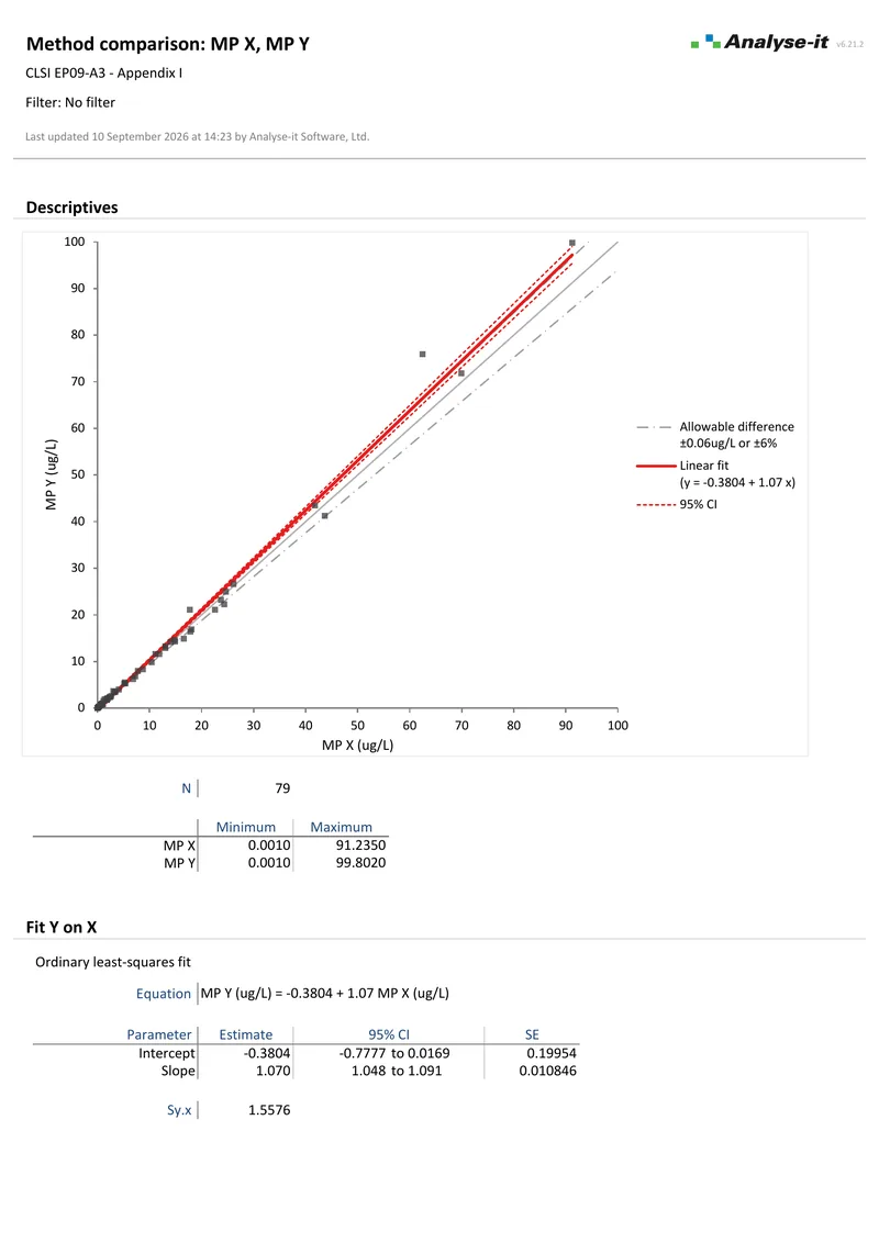
79 observations. OLS, Weighted OLS, Deming, Weighted Deming, and Passing-Bablok. Each with scatter plot, fit, and allowable difference. Bias at decision point 5 μg/L with CI and equality test.
EP21 A Example 1 EP21-A — Table 2
LDL cholesterol total analytical error.
100 observations. Bland-Altman with median bias, 95% limits of agreement, mountain plot, and allowable difference ±10 mg/dL.
EP21 A Example 2 EP21-A — Table 3
Sodium total analytical error.
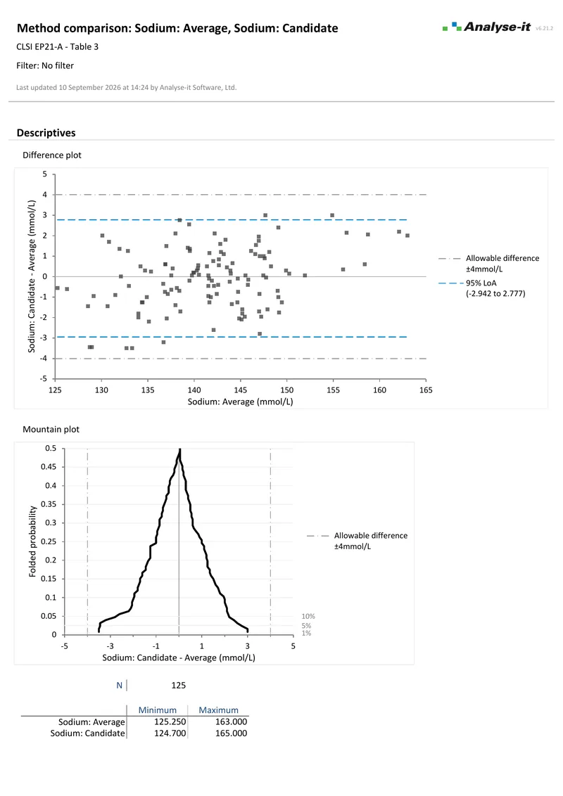
125 observations. Bland-Altman with mean bias, 95% limits of agreement with 90% CIs, mountain plot, and allowable difference ±4 mmol/L.

Part of the Method Validation Edition

Method comparison is one part of the Method Validation Edition, alongside measurement system analysis, reference intervals, and diagnostic performance.

Related guides in our Learn section: choosing a regression, Bland–Altman limits of agreement, bias at a medical decision point, how many samples you need, total analytical error, commutability, allowable total error, total error or measurement uncertainty, and comparing instruments within one laboratory.

Software you can trust

Validated calculations you can defend at inspection Every calculation is performed by Analyse-it — no Excel formulas, no third-party functions. Results are validated against CLSI reference datasets, published datasets, and thousands of internal test cases before every release. See how we develop and validate Analyse-it →
Data stays in your facility Analyse-it runs entirely within Microsoft Excel on your PC. No cloud processing, no data transmission. Pre-submission data, patient-adjacent data, and in-process results stay within your facility under your own data governance controls.
Standard Excel workbooks anyone can open Every analysis is an ordinary .xlsx workbook. Share with colleagues, submit to regulatory affairs, archive for audit, open on any PC with Excel. No proprietary format, no licence required to view results. Colleagues and auditors see exactly what you see.
Results that cannot be accidentally broken Analysis output contains computed values, not formulas. Nothing to accidentally overwrite, no cell references to break, no formula errors to introduce. The results you reported are exactly what you will find when you reopen the workbook months or years later for an audit.

Free trial and pricing

Try it on your own data first. The 15-day trial is every feature from all five editions, with no sign-up and no licence key — install it and start straight away.

Method Validation edition from US$ 475 per year, or US$ 1155 for a perpetual licence. Every purchase carries a 30-day money-back guarantee. Need a quote for purchasing? Add the licence to the cart and save it as a PDF quote.