
Learn how to verify that a measurement procedure meets performance requirements before introducing a new measurement procedure into the laboratory, after maintenance to the measuring system, or upon failing a proficiency test or inspection.
In this tutorial you will use the CLSI EP15-A3 procedure to verify the precision against the manufacturer’s claim and estimate the bias using proficiency testing materials.
Estimate the precision of the measurement procedure.
The variability plots show a simple visual assessment of the closeness of agreement between the measured quantity values. The purple lines show the mean of each run and the blue line the overall grand mean, allowing you to see the variation between and within each run.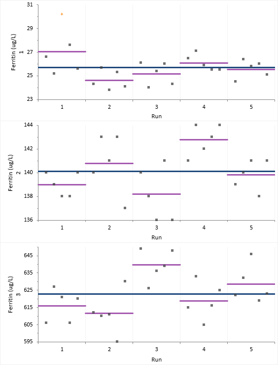
You should observe the scatter of the points to ensure there are no obvious problems. If a result appears spurious then you should investigate and correct any mistakes. If the data appear to be unusable, stop the evaluation and begin an expanded evaluation of the sources of measurement error or contact the manufacturer. We note that one observation in Sample 1, Run 1 is highlighted as a potential outlier but do not know the reason for the aberrant result. We will continue with this observation included in the analysis and return to it later.
The abbreviated variance components table shows precision expressed numerically as the standard deviation (SD) and coefficient of variation (CV).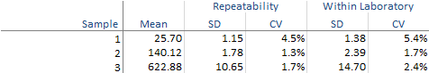
Test if the precision meets the manufacturer's performance claim.
You should use this procedure when you already have a performance claim from a manufacturer's package insert and you want to test whether your precision is significantly greater than the claim. It is possible for the imprecision from a study to be greater than the manufacturer's claim due to the chance alone. This procedure ensures that the manufacturer's claims are only falsely rejected 5% of the time when they are in fact true.
The detailed variance components table shows the observed and expected SD/CV along with the hypothesis test p-value for each level.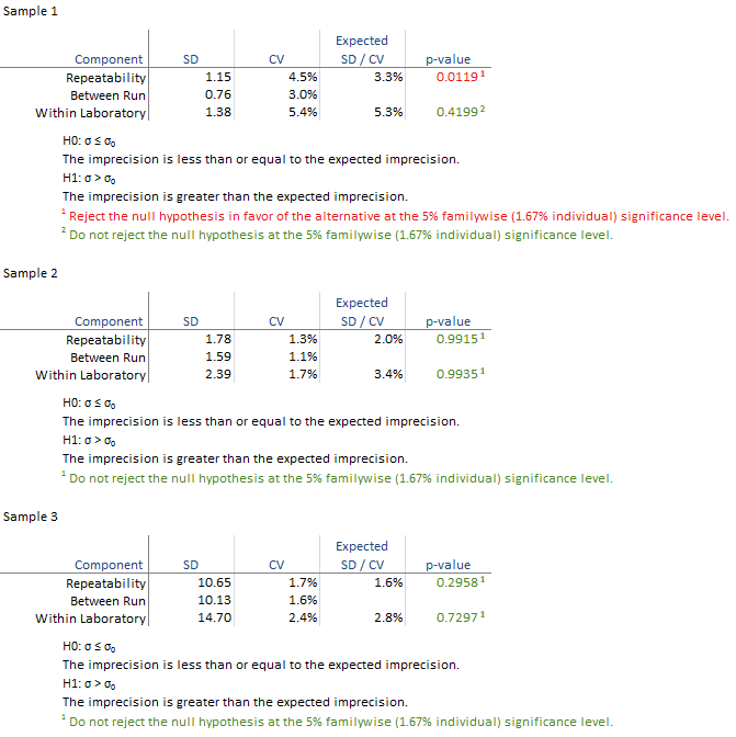
All the hypothesis tests are not significant and highlighted green in this example. If any are significant they are highlighted in red and you should contact the manufacturer for further assistance in diagnosing the problem. If the hypothesis test is not statistically significant but the imprecision estimate is much larger than the claim, you may want to repeat the study with more data to be able to detect smaller departures from the claim.
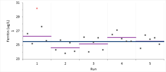
Dealing with outliers and assessing their impact.
Even after correcting or excluding all result known to be spurious, there may sometimes be results marked as statistical outliers. This may be due to a nonperformance-related cause, which, if known, would have justified excluding the result. Alternatively, the apparently extreme results may genuinely represent the performance. There is always a trade-off between retaining the result which will inflate the imprecision estimates, or exclude it which may overly optimistic estimates. It is often good practice to calculate the results before and after excluding the outlier.
The variability plot show the excluded observation as a red cross.
The detailed variance components table shows the observed and expected SD/CV along with the hypothesis test p-value for each level.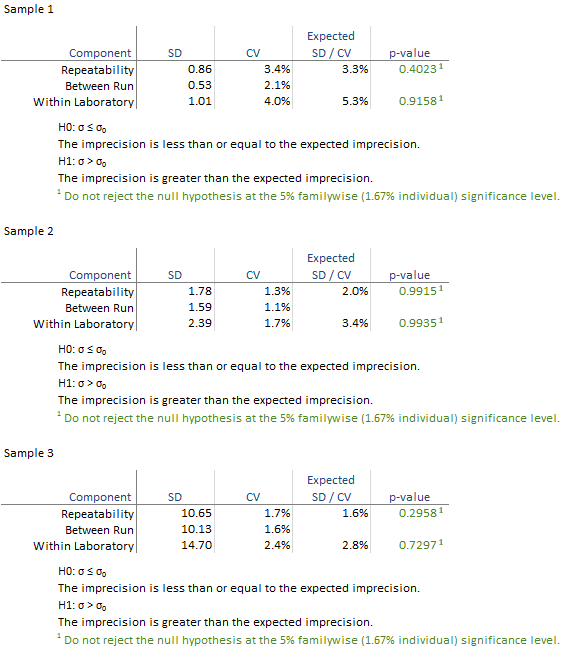
All the hypothesis tests are not significant and highlighted green. Because the exclusion of the outlier changes the outcome of the study it is essential to assess the clinical effect of the outlier and investigate further to try and determine its cause, or contact the manufacturer for further assistance in diagnosing the problem.
Estimate the bias using reference materials.
You should use this procedure when you already have a sample with a known assigned value and you want to estimate the bias and test whether it is significantly different to zero. It is possible for the bias from a study to be greater than zero due to the chance alone. This procedure ensures that the assumption that the bias is 0 is only falsely rejected 5% of the time when it is in fact true.
The table shows the observed and expected value along with the bias and the hypothesis test p-value for each level.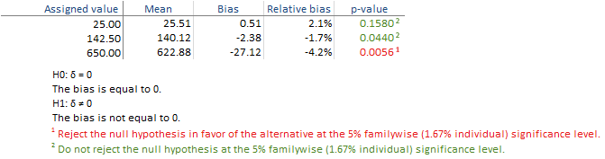
The hypothesis tests for level 1 and 2 are not significant in this example, but for level 3 the bias is significantly different from zero and is highlighted in red. You should therefore determine if the bias is acceptable for your laboratories needs by comparing it to user-specified allowable bias, or contact the manufacturer for further assistant in diagnosing the problem. If the hypothesis test is not statistically significant but the bias estimate is much larger than zero, you may want to repeat the study with more data to be able to detect smaller departures from the zero.