
Learn how to assess the agreement between two methods of measurement.
In a 1986 issue of The Lancet, Bland & Altman published a paper that changed how method comparison studies are performed. In 1999, they published a follow-up paper that extended their earlier work to many different scenarios.
If you prefer you can watch a video of this tutorial.
In this tutorial you will perform the following tasks:
When assessing the agreement between two methods, it is useful to the plot the difference between methods against the mean of the methods (a difference plot).
A difference plot is, effectively, a scatter plot rotated 45 degrees clockwise. However, a difference plot is more informative than a scatter plot since the data points are not tightly clustered around the diagonal. A difference plot also clearly shows any relationship between the differences and the magnitude of measurement.
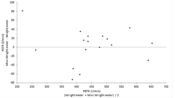
To illustrate this concept, we will use an example from Bland & Altman’s 1986 paper. This example compares two methods of measuring peak expiratory flow rate (PEFR). On each of 17 subjects, two measurements were taken with a Wright meter, and two with a mini Wright meter.
The points on the difference plot roughly form a constant width horizontal band across the measuring interval, and there is no obvious relationship between the difference and the mean or the variability of the measurements and the mean.
If the differences are not related to magnitude, the mean of the differences provides an estimate of the average bias between the methods. The limits of agreement estimate the interval that a given proportion of differences between measurements is likely to lie within. The limits can be used to determine if the methods can be used interchangeably, or if a new method can replace an old method without changing the interpretation of the results.
The mean difference estimate is 2.1, which indicates that the Mini Wright meter reads on average 2.1 l/min higher than the Wright meter. A hypothesis test could be performed to determine if this is significantly different from zero. If it is, adjusting readings from the Mini Wright meter by subtracting 2.1 will make them agree more closely with the Wright meter.

The limits of agreement estimate an interval of -73.9 to 78.1, which indicates that the Mini Wright meter may measure as much as 73.9 l/min below and 78.1 l/min above the large meter. This would be unacceptable for clinical purposes.
The confidence intervals for the mean difference and limits of agreement indicate the uncertainty in the estimates. The wide intervals are due to the small sample size and large variation of the differences. Even the most optimistic interpretation would conclude that the agreement is unacceptable.
Repeatability — or variation in repeated measurements on the same subject under identical conditions over a short period of time — is important because it directly affects the agreement between methods. To assess repeatability, two or more measurements by each method on each subject must be made.
If one method has poor repeatability, the agreement between the two methods will also be poor. If both methods have poor repeatability, the agreement will be even worse. When comparing agreement with an old method with poor repeatability, even a perfect new method will not agree with it.
The repeatability plots show the standard deviation (SD) of the measurements for each subject and method. Larger values indicate poor agreement between replicate measurements. Based on the plots, the repeatability of both methods is similar and the SD is not related to the magnitude of the measurement.
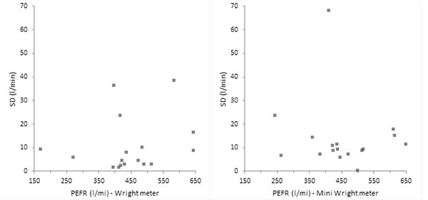
The coefficient of repeatability is 42.4 for the Wright meter and 55.2 for the Mini Wright meter. Therefore, 95% of differences between repeated measurements made with the Wright meter are expected to be within 42.4 l/min and similarly 55.2 l/min for the Mini Wright meter.
When repeated measurements (replicates) are made for each subject, it is inefficient to estimate average bias and limits of agreement using only the first measurement, rather than all measurements.
If replicates are available, it is sensible to use the mean of the replicates to estimate average bias. However, when estimating the limits of agreement, the reduction in the standard deviation due to averaging of the measurements must be considered and adjusted for if necessary.
The mean difference estimate is 6.0, which indicates that the Mini Wright meter reads on average 6.0 l/min higher than the Wright meter. The confidence interval is narrower because the measurement error was reduced by using the mean of the replicates.

The limits of agreement estimate an interval of -67.8 to 79.8, which indicates that the Mini Wright meter may measure as much as 67.8 l/min below and 79.8 l/min above the large meter. This would be unacceptable for clinical purposes. Again, the confidence intervals are narrower due to the use of more measurements.
The difference plot may sometimes suggest a relationship between the differences and magnitude of measurement. Often, the band of points on the difference plot will start narrow and then widen to the right of the plot as magnitude increases. This indicates that the variability of the differences increases with magnitude of measurement. Sometimes, the band of points may not be horizontal, which indicates a relationship between average difference and the magnitude.
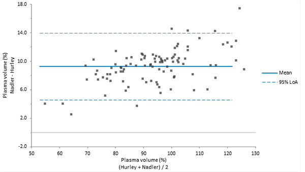
To illustrate these concepts, we will use an example from Bland & Altman’s 1999 paper. This example measures plasma volume expressed as a percentage of normal using two alternative sets of normal values from Nadler and Hurley.
The difference plot shows an obvious systematic difference between the methods as all the differences are above the line of equality (zero). There is also a clear relationship between the difference and the mean, with the difference increasing as plasma volume rises. The limits of agreement appear rather wide at low values and too narrow at higher values.
When the differences are related to magnitude, it is best to try to eliminate the relationship using a transformation. Because it has a clear interpretation, logarithmic transformation is often used to remove the effect of differences increasing with magnitude. (The difference between the logarithms of two values is equivalent to the ratio of the two values.)
Other transformations, such as square root or reciprocal, cannot be clearly interpreted and are best avoided. However, rather than use a logarithmic transformation, it is usually easier to use the ratio of the measurements or the difference expressed as a percentage of the mean.
The difference plot shows the ratio of the measurements with the points now forming a constant-width band across the measuring interval.
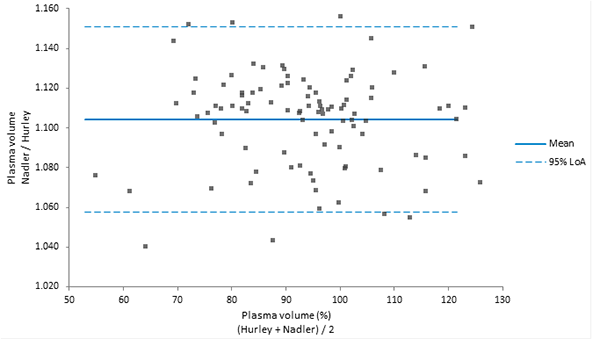
The mean ratio estimate is 1.10, which indicates that the Nadler method measures an average of 10% higher than the Hurley method. The limits of agreement indicate that the Nadler method may measure between ~6% to ~15% above the Hurley method for 95% of measurements.

Sometimes, a transformation does not solve the problem of a relationship between the differences and magnitude. For example, this could occur when differences are negative for low values and positive for high values.
To illustrate these concepts, we will use another example from Bland & Altman’s 1999 paper. In this example, the fat content of human milk was measured by enzymic procedures for the determination of triglycerides and using the standard Gerber method.
The difference plot shows the average bias estimated using a linear regression. The limits of agreement are estimated using the residual standard deviation from the regression.
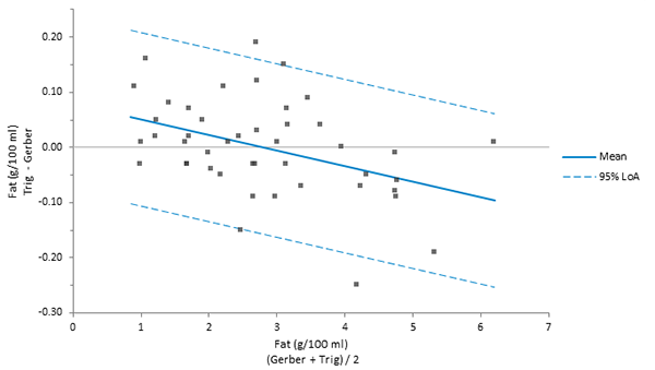
The p-value of the slope term is significant (p < 0.05) and confirms that the average difference is related to the magnitude.
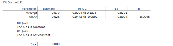
If we suspect that the variability of the differences is also related to the mean, we could model the SD using the residuals from the fit.
An assumption of the Bland-Altman limits of agreement is that the differences (or residuals, when fitting a regression) are normally distributed. In many cases, there will not be a big impact on the limits of agreement when the distribution of the differences is not normal. However, there may be cases where it is preferable to estimate the limits using a nonparametric method.
A histogram of the differences is useful for assessing the assumption of normality. If the distribution is skewed or has very long tails, the assumption of normality may not be valid.
To illustrate these concepts, we will use another example from Bland & Altman’s 1999 paper. This example shows the differences in systolic blood pressure measurements by a device and those by sphygmomanometer.
The difference plot shows the limits of agreement estimated using the 2.5th and 97.5th percentiles and the average bias estimated as the median of the differences.
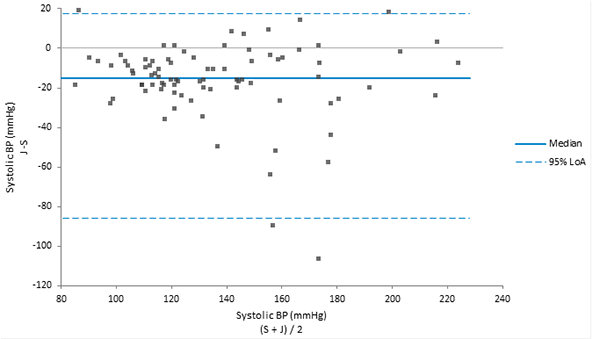
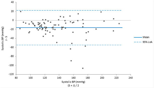
The limits of agreement estimated by the nonparametric method are wider than the limits estimated using the parametric method. Roughly 2.5% of the observations are above, with a similar percentage below the limits of agreement. In contrast, the narrower parametric-based limits of agreement show all observations outside the lower limits of agreement and none above the upper limit.