Every feature from all five editions for 15 days.
Medical edition from US$ 340 a year · 30-day money-back guarantee.
Excel’s PERCENTILE function returns a quantile and stops. No confidence interval on the limit, no choice of quantile method for the sample size, no transformation for skewed data, no partition by sex or age. Every laboratory result a clinician sees is interpreted against a reference interval. Normal patients are flagged and abnormal patients are missed when the interval is wrong. Wrong can mean too wide, too narrow, from the wrong population or not partitioned where it should be.
Which quantile method suits this sample size and distribution? Should the interval be partitioned by sex or age? Establishing intervals from your own population is one of the most consequential statistical tasks a laboratory performs.
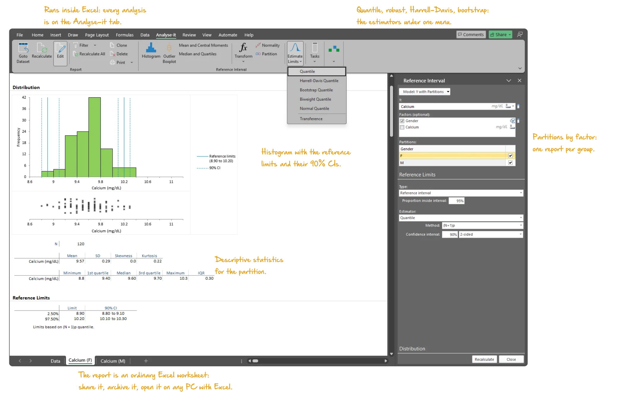
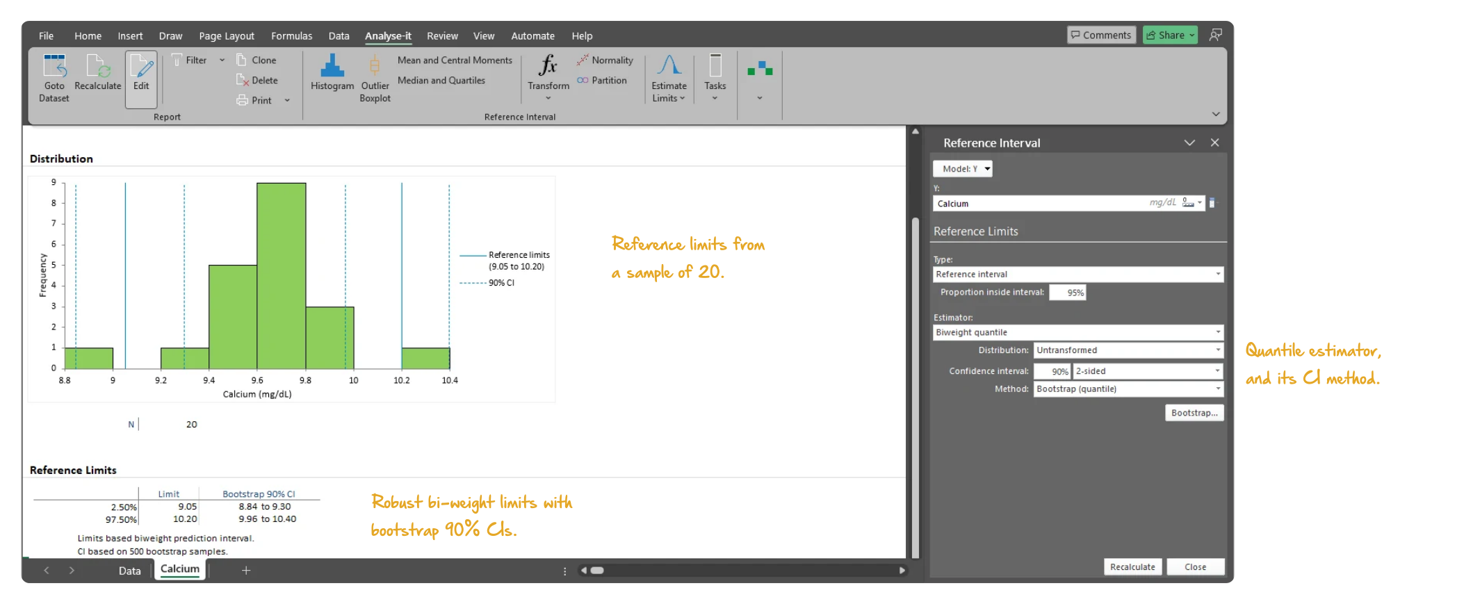
The quantile method should match the sample size and the shape of the data. Parametric quantiles when the distribution is Gaussian. Non-parametric with three computation approaches — (N+1)p, Np+½ and (N+⅓)p+⅓ — when there are 120 or more observations. Robust bi-weight for small or moderately skewed samples, bootstrap for distribution-free estimation, Harrell-Davis for a smooth quantile estimate. Every reference limit has a confidence interval, and the frequency histogram shows the limits against the data.
Where a reference interval differs between subgroups, one interval for everyone misclassifies patients in both. Partition by sex, age group, ethnicity or any combination of factors within a single analysis. Separate calcium intervals for males and females, for example, or age-stratified alkaline phosphatase ranges for paediatric populations. Outlier screening and normality assessment run independently for each subgroup.
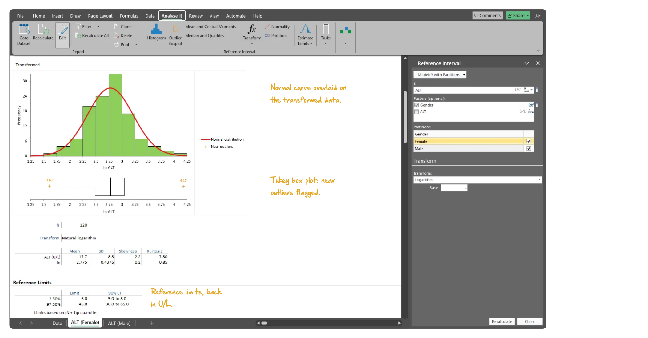
Non-normal data forced through a parametric calculation gives limits that do not fit the population. Log, square root, cube root, reciprocal, Box-Cox, Manly exponential and two-stage exponential/modulus transformations bring skewed data closer to normal. Choose the transformation that achieves the best fit, compute parametric reference limits on the transformed scale and back-transform to the original units.

An extreme value or a wrong assumption about the distribution distorts the limits, so screen the data before establishing them. The Tukey box plot identifies outliers. Normality is assessed with the Shapiro-Wilk and Anderson-Darling tests, the frequency histogram with normal overlay and the normal Q-Q plot with Lilliefors confidence band. Run them on the raw data, and again after a transformation.
See reference interval results in detail — partitioned intervals, histograms with reference limits and outlier screening — using example datasets you can download and follow along with.
Reference intervals are one part of the Medical edition, alongside diagnostic accuracy, Bland-Altman agreement and survival analysis. The edition also includes the full Standard edition for hypothesis testing, regression and descriptive statistics.
Related guides in the Learn section: choosing a reference interval method, transferring and verifying an interval, when to partition and handling outliers and skew.
For the rest of a method validation programme — precision, linearity, detection limits, bias at clinical decision points, regression-based method comparison and reference-interval transference — see the Method Validation edition.
Try it on your own data first. The 15-day trial is every feature from all five editions — install it and start straight away.
Medical edition: US$ 340 per year or US$ 815 for a perpetual licence. Every purchase carries a 30-day money-back guarantee. Need a quote for purchasing? Choose the licence on the pricing page and click Get a quote.