Examples Fifty worked analyses, each with the data behind it. Open the PDF to see the analysis as Analyse-it produces it, or open the workbook in the software to change it.

Every example is a real analysis of a real dataset. Use one as a template. The workbook shows how to arrange your data, and the analysis can be reopened and edited if you have the Analyse-it edition it needs.

Each card links to the analysis as a PDF and to the workbook as an XLSX. The workbooks were saved with Analyse-it 6.21 — see the release history.

Without a licence, the free 15-day trial opens every one of them.

Method validation

Precision, trueness, linearity, detection capability and method comparison, worked to the CLSI protocol or published method each one follows. 17 examples

Glucose precision report 1 page EP05-A2 — Appendix B
Glucose precision, single site.
20 days × 2 runs × 2 observations, 80 results. Variability plot, then repeatability, between-run, within-day, between-day and within-laboratory components with CIs and the ANOVA table with expected mean squares. Method Validation
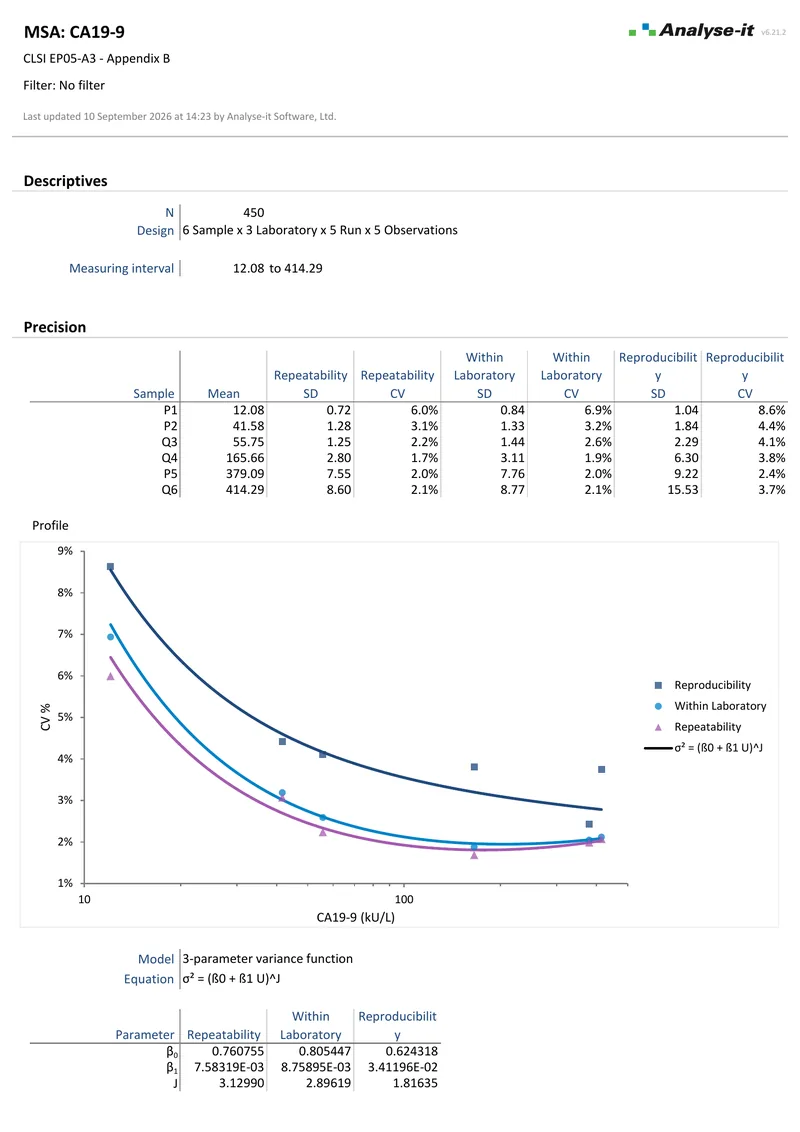
CA19-9 precision report 3 pages EP05-A3 — Appendix B
CA19-9 precision, multi-site.
6 samples × 3 laboratories × 5 runs × 5 observations, 450 results. Repeatability, within-laboratory and reproducibility for each sample, then a precision profile fitted with a three-parameter variance function. Method Validation
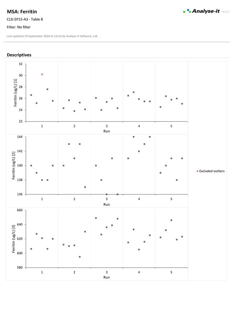
Ferritin precision verification report 3 pages EP15-A3 — Table 8
Ferritin precision verification.
3 samples × 5 runs × 5 observations. Outlier identification with the flagged results excluded, then a variability plot and within-run and total precision. A χ² test of each against the manufacturer’s claim at a 1.67% individual significance level. Method Validation
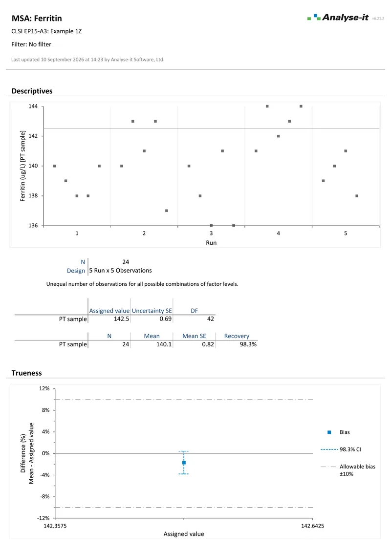
Ferritin trueness verification report 2 pages EP15-A3 — Example 1Z
Ferritin trueness verification.
5 runs × 5 observations against a proficiency testing sample with an assigned value of 142.5 and a stated uncertainty. Recovery, bias with a 98.3% CI against an allowable bias and a t test of the bias. Method Validation
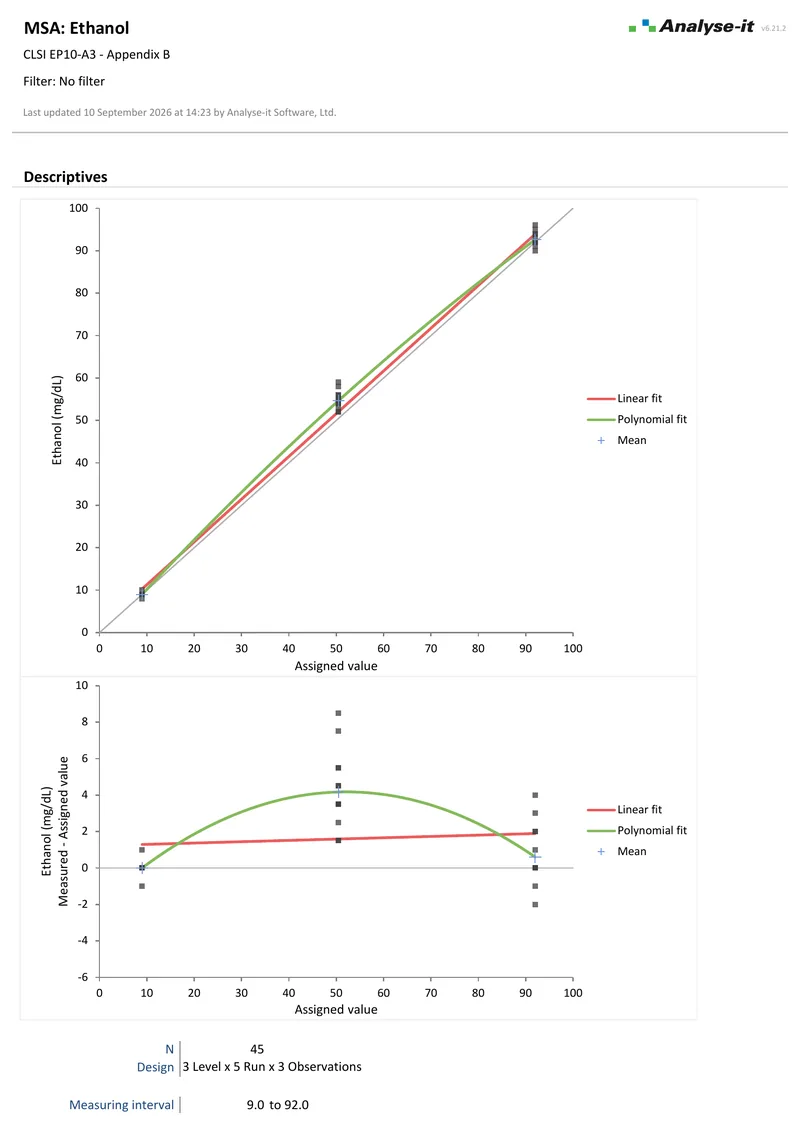
Ethanol preliminary evaluation report 3 pages EP10-A3 — Appendix B
Ethanol preliminary evaluation.
3 levels × 5 runs × 3 observations. Precision at each level against an allowable goal, where the mid level fails and a precision profile. Bias at each assigned value on a difference plot with allowable bias bands, then linear and second order fits across the measuring interval. Method Validation
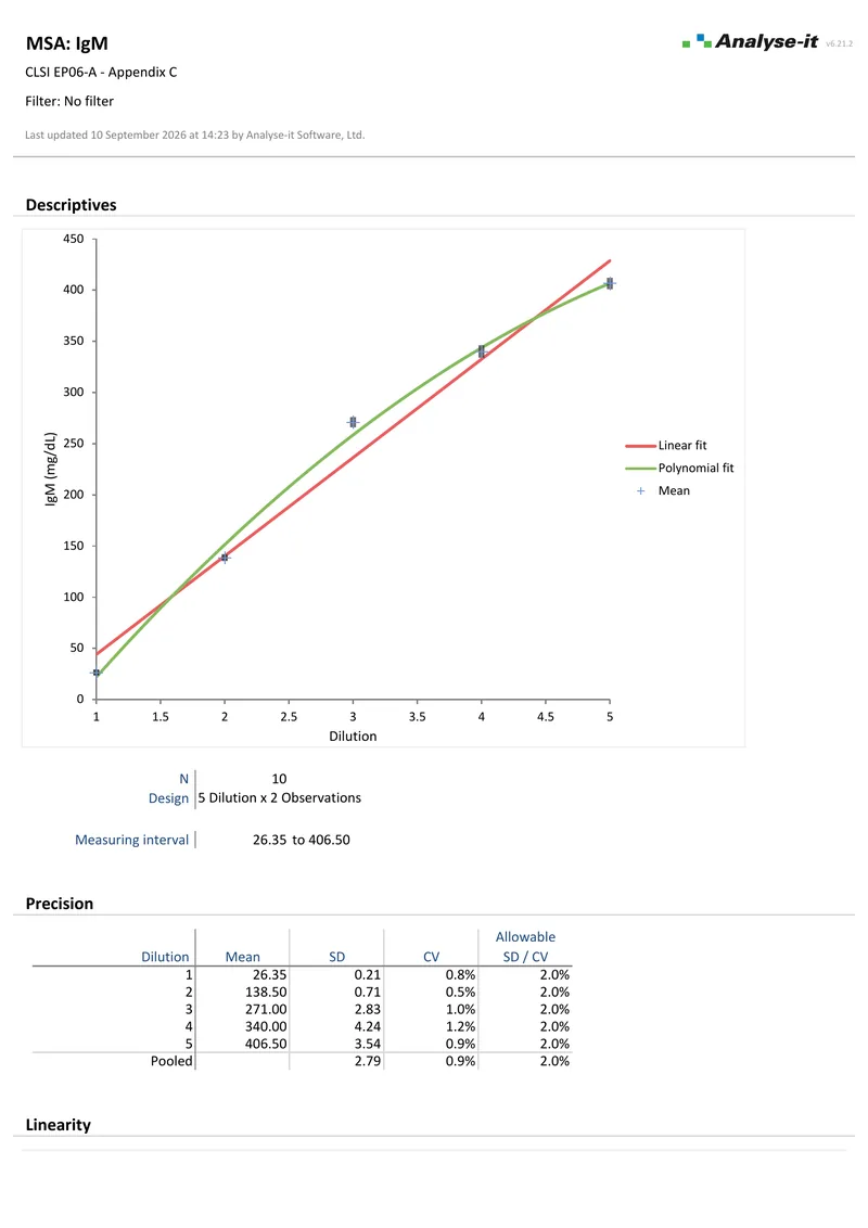
IgM linearity report 3 pages EP06-A — Appendix C
IgM linearity.
5 dilutions × 2 observations. Linear, second and third order polynomial fits, then nonlinearity at each dilution with 95% CIs against a ±5% allowable band, and a difference plot. Only dilution 4 meets the requirement. Method Validation
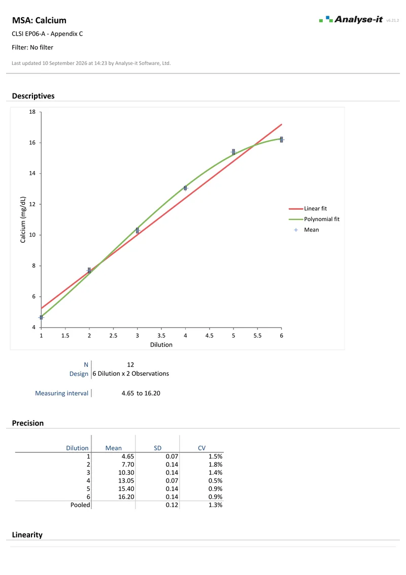
Calcium linearity report 6 pages EP06-A — Appendix C
Calcium linearity, full and reduced interval.
6 dilutions × 2 observations. Over the full interval five of the six dilutions exceed the ±0.2 mg/dL allowable nonlinearity, so a second analysis refits over a reduced interval that passes throughout. Linear and polynomial fits with nonlinearity at each dilution. Method Validation
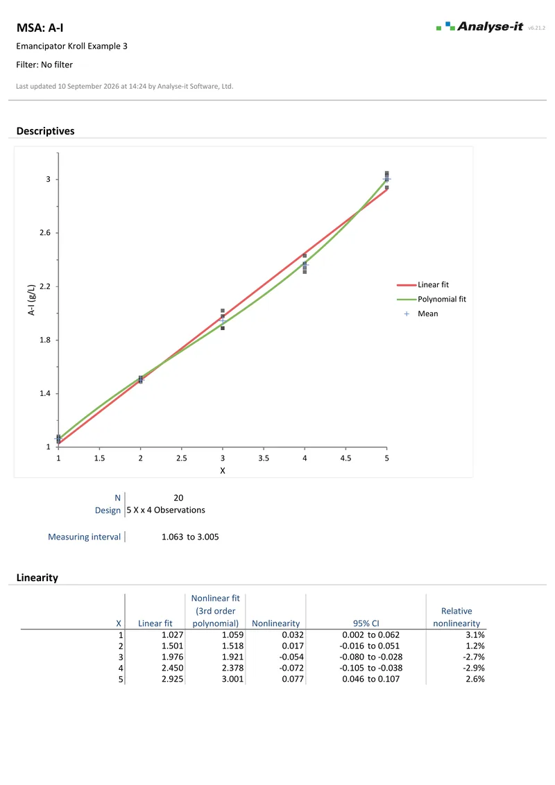
Linearity with lack-of-fit test report 2 pages Emancipator and Kroll, example 3
Linearity with a lack-of-fit test.
5 concentrations × 4 observations. Linear fit with an F test for lack of fit against pure error. Then a third order polynomial fit and nonlinearity at each level expressed relative to the fitted value. Method Validation
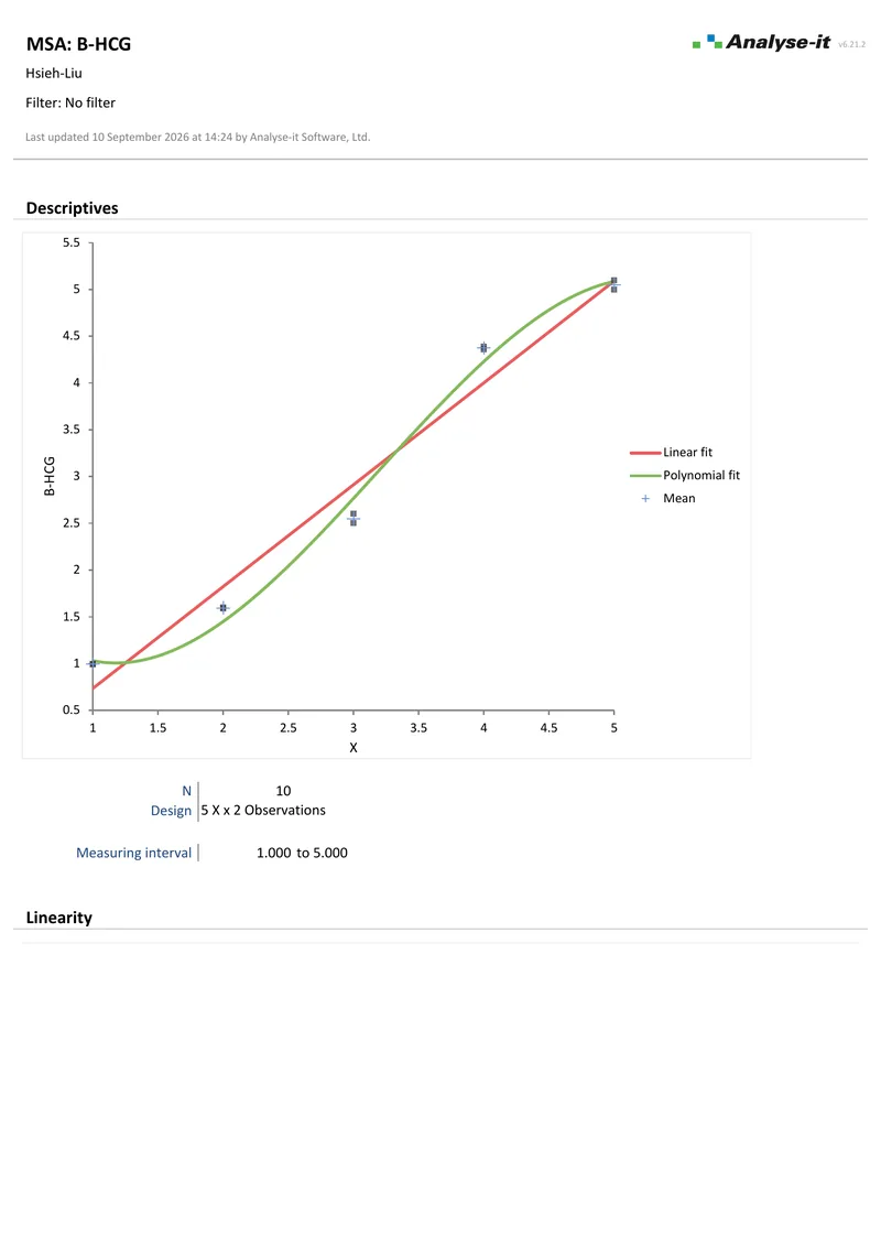
Linearity equivalence test report 3 pages Hsieh and Liu
β-HCG linearity by equivalence testing.
5 concentrations × 2 observations. Linear, second and third order fits, each with a lack-of-fit test. Then a two one-sided test of the difference between the linear and nonlinear fit against the allowable nonlinearity. Method Validation
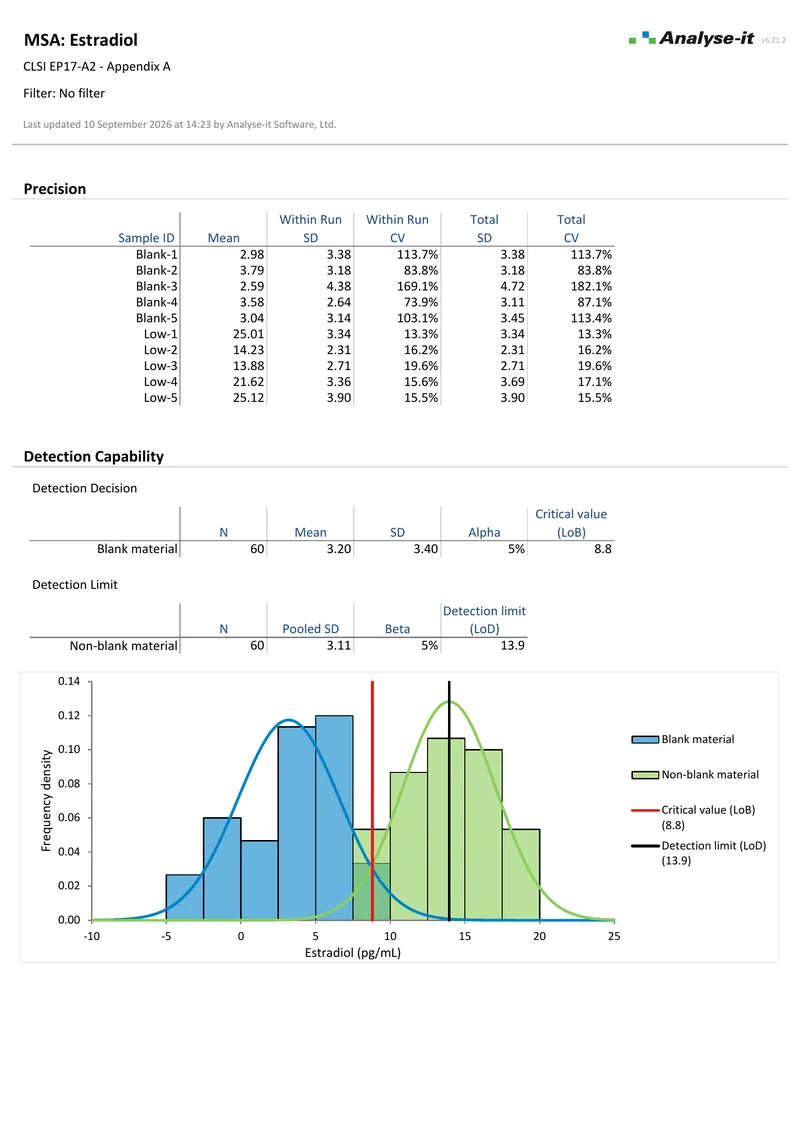
Estradiol detection capability report 2 pages EP17-A2 — Appendix A
Estradiol detection capability, two reagents.
5 blank and 5 low-level samples per reagent, 60 results each. Within-run and total precision for every sample, the limit of blank from the blank distribution and the limit of detection from the pooled SD of the low-level samples. A bi-histogram sets the blank against the low-level material. Method Validation
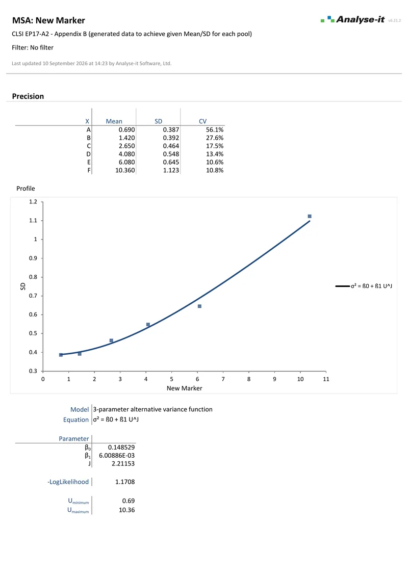
New Marker limit of detection report 4 pages EP17-A2 — Appendix B
New Marker, limit of detection from a precision profile.
Six pools per reagent across the measuring interval. The profile is fitted with a three-parameter alternative variance function for one reagent and a mixed constant and proportional function for the other. The limit of detection is then read from the profile against a known limit of blank. Method Validation
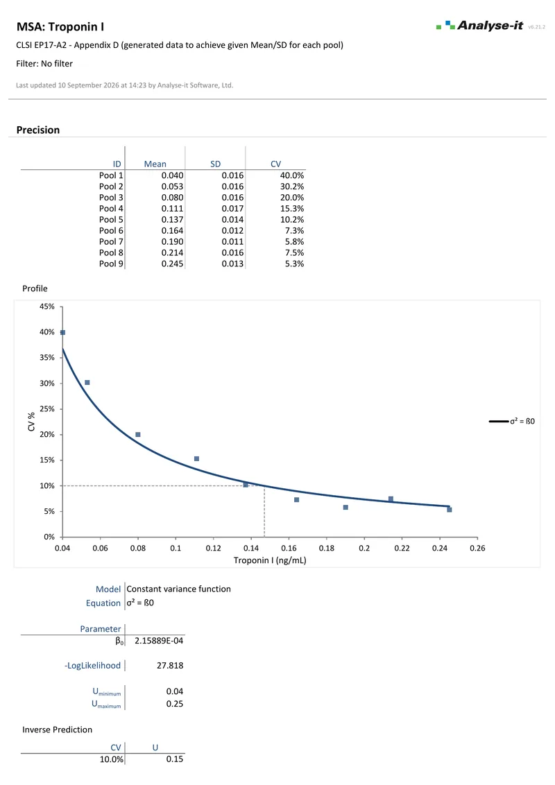
Troponin I limit of quantitation report 2 pages EP17-A2 — Appendix D
Troponin I, limit of quantitation.
Nine pools per reagent, 720 results each. Precision profile fitted with a constant variance function, then inverse prediction of the concentration at which the CV meets the goal — the limit of quantitation. Method Validation
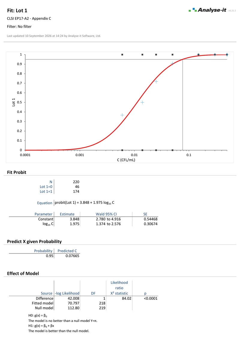
Probit analysis detection capability report 3 pages EP17-A2 — Appendix C
Detection capability by probit analysis.
A dilution series of detected and not-detected results, fitted separately for three reagent lots. Probit regression against log concentration with parameter estimates and Wald CIs, a likelihood ratio test for the model and the concentration detected with 95% probability. Method Validation
Partitioned difference plot report 2 pages EP09-A3 — Appendix I
Difference plots over a partitioned interval.
79 observations split at 1.8 µg/L, 40 below and 39 above. Each interval gets its own difference plot, mean difference with a 95% CI and a hypothesis test. The allowable difference is ±0.06 µg/L below the split and ±6% above it. Neither interval shows a significant bias. Method Validation
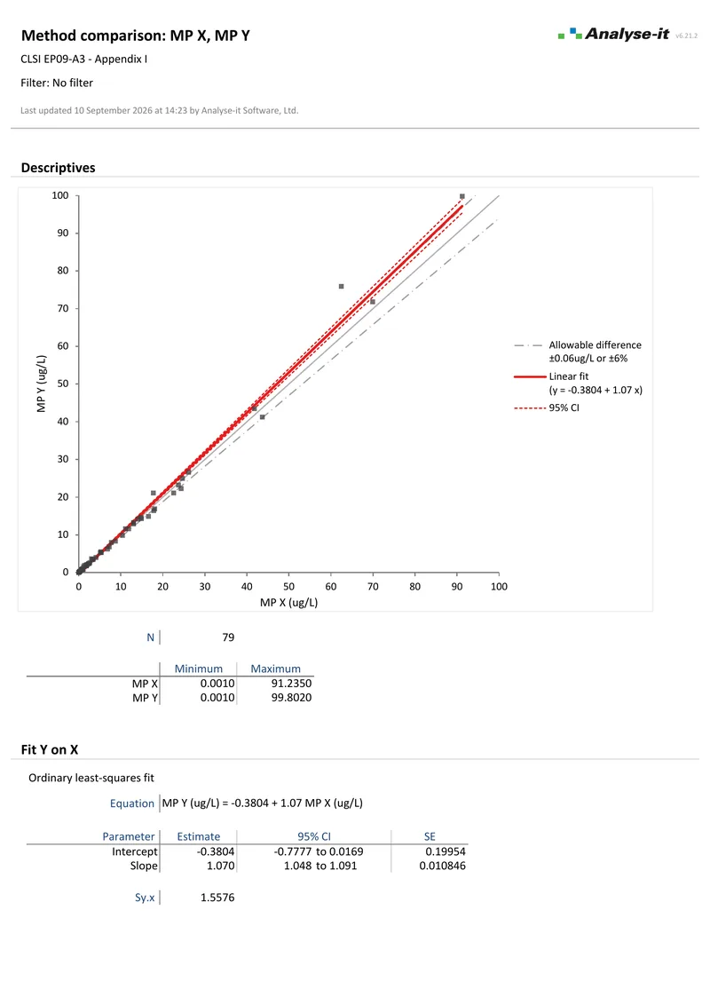
Five method comparison regression fits report 10 pages EP09-A3 — Appendix I
All five regression fits.
79 observations fitted five ways — ordinary least squares, weighted least squares, Deming, weighted Deming and Passing-Bablok. Each analysis gives the equation, parameter estimates with CIs and the predicted bias at a medical decision point of 5 µg/L. Weighted least squares is the fit that misses the allowable difference. Method Validation
LDL cholesterol total analytical error report 2 pages EP21-A — Table 2
LDL cholesterol total analytical error.
100 observations. Difference plot and mountain plot with an allowable difference of ±10 mg/dL, median difference with a 90% CI and 95% limits of agreement. Method Validation or Medical
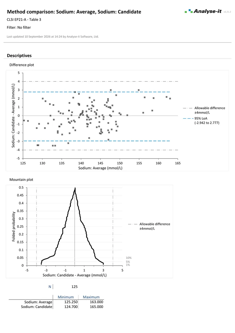
Sodium total analytical error report 2 pages EP21-A — Table 3
Sodium total analytical error.
125 observations. Difference plot and mountain plot with an allowable difference of ±4 mmol/L, mean difference with a 90% CI and 95% limits of agreement, each with their own CI. Method Validation or Medical

Diagnostic performance and reference intervals

Judging how well a test separates the diseased from the well, and establishing the interval a result is read against. 8 examples

ROC curve analysis report 2 pages EP24-A2 — Appendix D
OxLDL and LDL diagnostic accuracy.
50 subjects, 28 of them with the condition. ROC curves for both markers with AUC, CIs and a test against 0.5 — OxLDL 0.80, LDL 0.56 — and a DeLong comparison of the two curves. A second analysis adds the bi-histogram and decision threshold plot for OxLDL alone. Method Validation or Medical
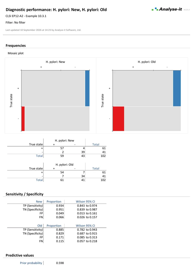
Qualitative test evaluation report 2 pages EP12-A2 — Example 10.3.1
H. pylori, two qualitative tests against a known state.
102 subjects. Mosaic plots, sensitivity and specificity with Wilson 95% CIs and predictive values at the observed prior. The difference between the two tests with Newcombe CIs and a score Z test. Method Validation or Medical
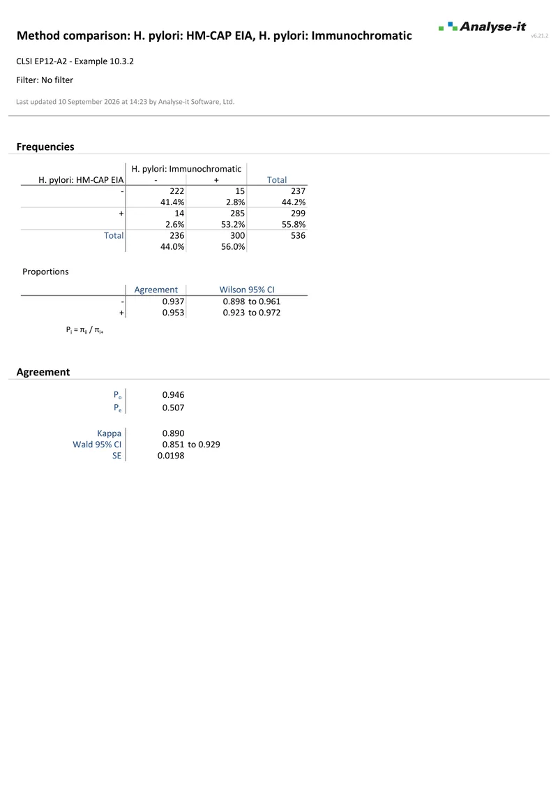
Qualitative method agreement report 1 page EP12-A2 — Example 10.3.2
H. pylori, agreement without a reference method.
536 samples compared between two qualitative methods with no true state available. Positive and negative agreement with Wilson CIs, overall agreement and Cohen’s kappa with a Wald 95% CI. Method Validation or Medical
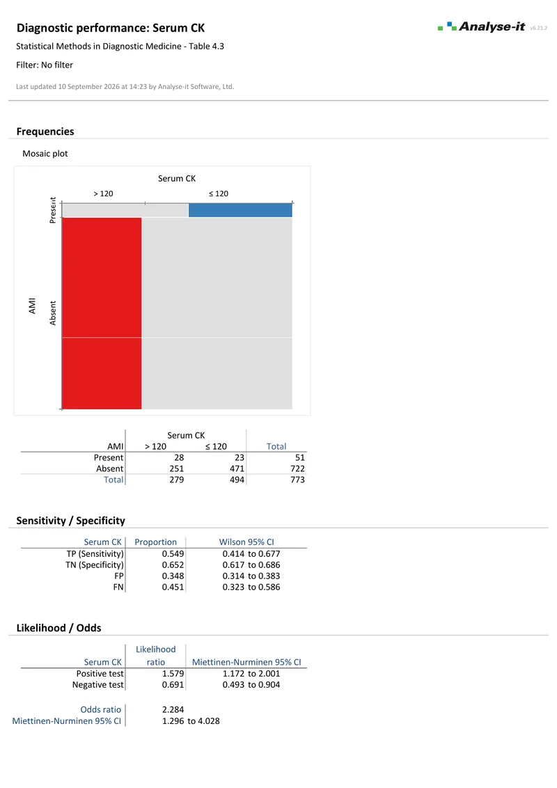
Serum creatine kinase diagnostic performance report 2 pages Serum creatine kinase for acute myocardial infarction
Statistical Methods in Diagnostic Medicine, table 4.3.
773 subjects at a fixed 120 U/L cut-off. The 2×2 table with a conditional odds ratio, exact CI and Fisher test. Then sensitivity and specificity with Wilson CIs, likelihood ratios with Miettinen-Nurminen CIs and a mosaic plot. Method Validation or Medical
Calcium reference intervals report 2 pages EP28-A3c — Table 4
Calcium reference intervals by sex.
120 observations per sex, reported separately. Distribution with descriptive statistics, and nonparametric reference limits from the (N+1)p quantile with 90% CIs. Method Validation or Medical
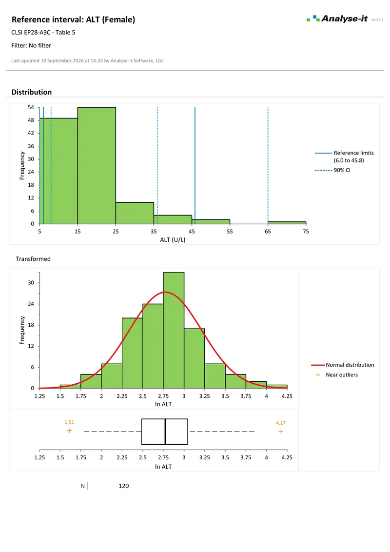
ALT reference intervals report 4 pages EP28-A3c — Table 5
ALT reference intervals by sex.
120 observations per sex, both skewed. A natural log transform, then nonparametric reference limits from the (N+1)p quantile with 90% CIs on the transformed scale. Method Validation or Medical
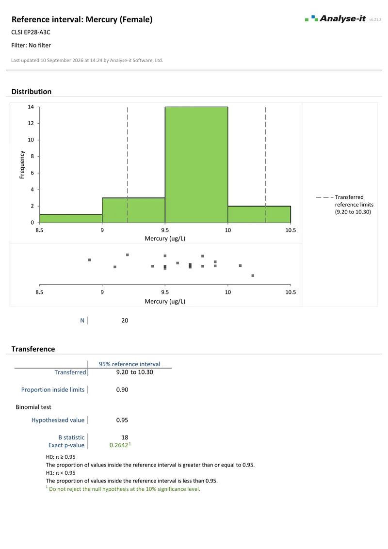
Reference interval transference report 2 pages EP28-A3c
Mercury reference interval transference.
20 observations per sex, tested against limits transferred from another laboratory. The proportion of results falling inside the transferred interval, with an exact binomial test against 95%. Method Validation
Robust reference interval report 1 page EP28-A3c — Appendix B
Calcium reference interval, robust method.
20 observations. Reference limits from the robust bi-weight prediction interval, with bootstrap 90% CIs from 500 samples. Method Validation or Medical

Quality control

Control charts for variables and attributes, process capability against a specification and Pareto analysis of causes. 6 examples

Shewhart, EWMA and CUSUM control charts report 6 pages Shewhart, EWMA and CUSUM
Copper concentration in a plating pool.
Three analyses on one dataset across the IQ, OQ and production phases. Xbar-R with Montgomery rules 1, 2, 3, 5 and 8 and points coloured by operator, flagging seven signals. EWMA with λ = 0.2 and L = 3 flags eight, and CUSUM with h = 5 and k = 0.5 flags eleven. Every signal falls in the IQ phase but one. Quality Control & Improvement
Individual and moving range chart report 2 pages Individual and moving range
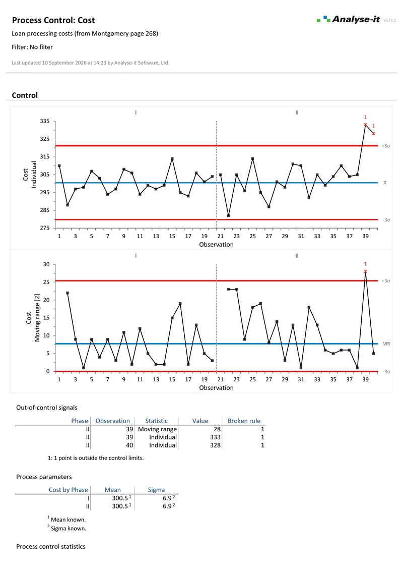
Loan processing costs.
Montgomery, page 268. 40 observations over two phases with a known mean and sigma. I-MR chart with ±3 sigma limits, flagging observation 39 on both charts and observation 40 on the individuals chart. Quality Control & Improvement
u chart report 1 page u chart
Supply chain errors per unit.
Montgomery, page 325. 20 samples of 50 units. u chart with ±3 sigma limits around a process mean of 0.074 errors per unit. No out-of-control signals. Quality Control & Improvement
p chart and standardised p chart report 2 pages p chart and standardised p chart
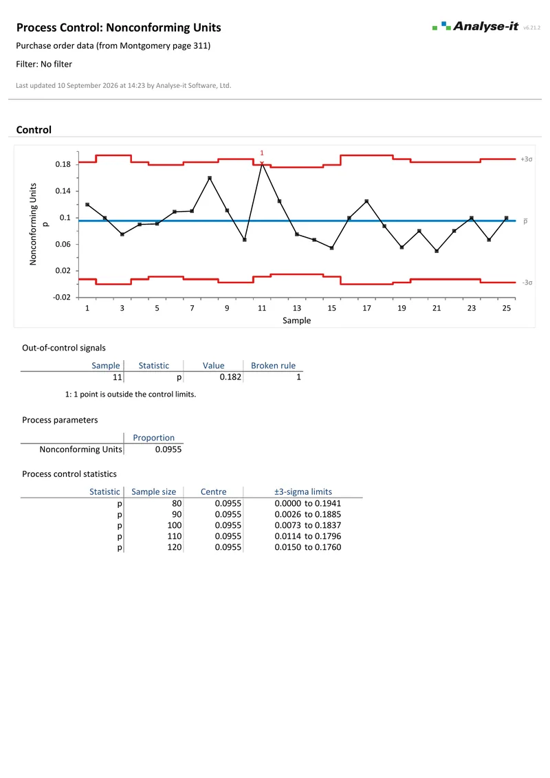
Nonconforming purchase orders.
Montgomery, page 311. 25 samples of varying size. A p chart whose limits move with the sample size, and the same data as a standardised Z-score chart with fixed ±3 limits. Sample 11 is out of control on both. Quality Control & Improvement
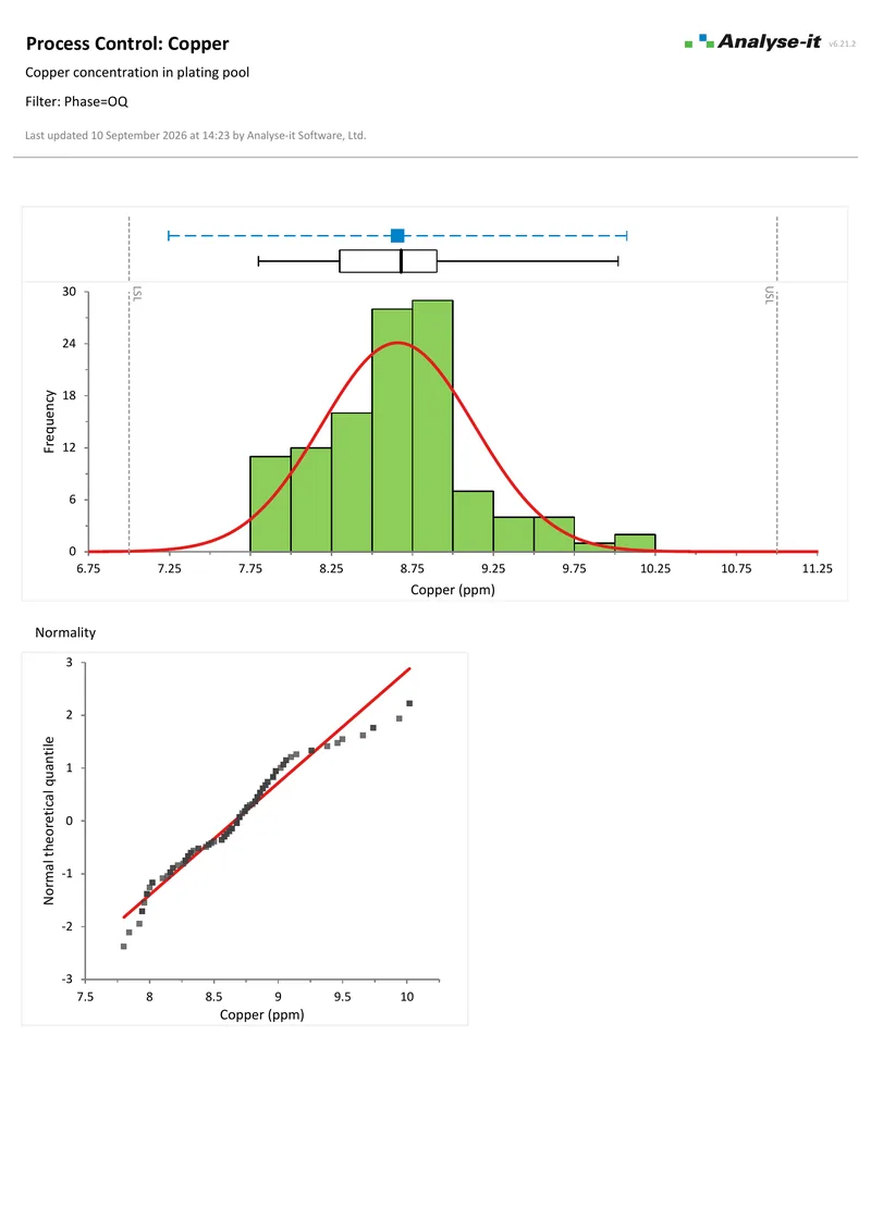
Process capability report 3 pages Process capability
Copper concentration against a 7 to 11 ppm specification.
The OQ phase only. An Xbar-R chart with Montgomery rules confirms the process is in control. Then a histogram with the specification limits, a box plot, a Q-Q plot and the Shapiro-Wilk test. Pp, Ppl, Ppu and Ppk with 95% CIs, expected nonconforming units at 216 PPM and Z benchmarks. Quality Control & Improvement
Pareto analysis report 3 pages Pareto analysis
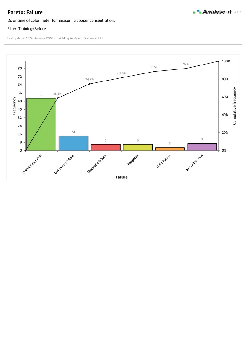
Colorimeter downtime before and after training.
Three analyses. A comparative Pareto stratified by three operators and by training status. Then a Pareto for the 87 failures before training and one for the 58 after, each ranking six failure categories with a cumulative line. Quality Control & Improvement

Distribution and comparing groups

Describing one variable, comparing two or more groups or conditions and testing association in a contingency table. 11 examples

Continuous distribution report 4 pages Continuous distribution
Newcomb’s speed of light, 64 observations.
Descriptive statistics, frequency histogram with custom classes, box and dot plot, cumulative distribution plot, normal Q-Q plot, Shapiro-Wilk normality test and a one-sample t-test against a hypothesised 29.97. A second analysis shows the frequency distribution on its own. Standard
Discrete distribution report 2 pages Discrete distribution
Hair and eye colour, 592 observations.
Frequency table with relative and cumulative frequency, a frequency plot and a whole-to-part plot and a Pearson χ² test of the observed proportions against a hypothesised distribution. Standard
One-way ANOVA report 3 pages One-way ANOVA
Y by brand, 7 groups, 19 observations.
Descriptive statistics by group, Levene test for homogeneity of variance, one-way ANOVA, Tukey-Kramer all-pairs comparisons over 21 contrasts with simultaneous 95% CIs and a Mean-Mean scatter plot. Standard
Independent-samples t-test report 2 pages Independent-samples t-test
Calcium supplementation and blood pressure, 21 observations.
Five-number summary by group with side-by-side plots, Fisher F test for the variance ratio, and Student’s t test of the difference in means against a hypothesised difference of 3. Standard
Compare pairs report 2 pages Compare pairs
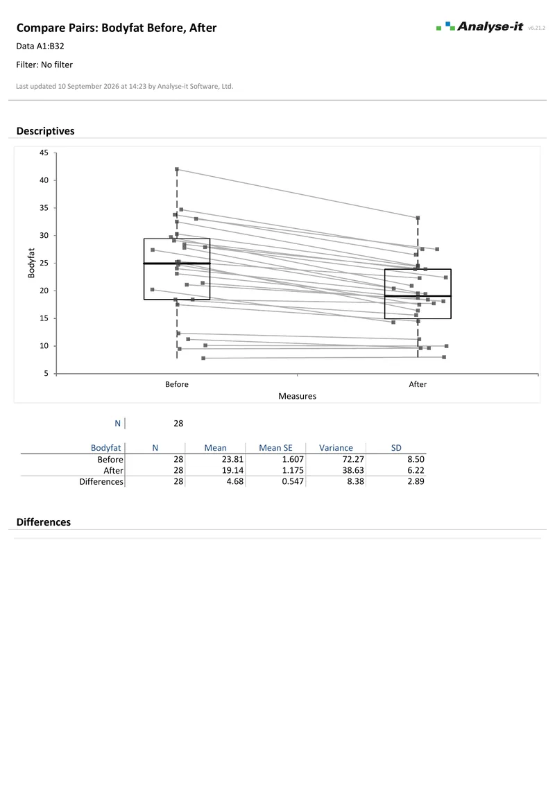
Body fat before and after an exercise programme.
28 paired observations. Descriptive statistics for both conditions and for the differences, Hodges-Lehmann shift estimate with a 95.49% CI and the Wilcoxon signed-ranks test. Standard
Independent contingency table report 2 pages Independent contingency table
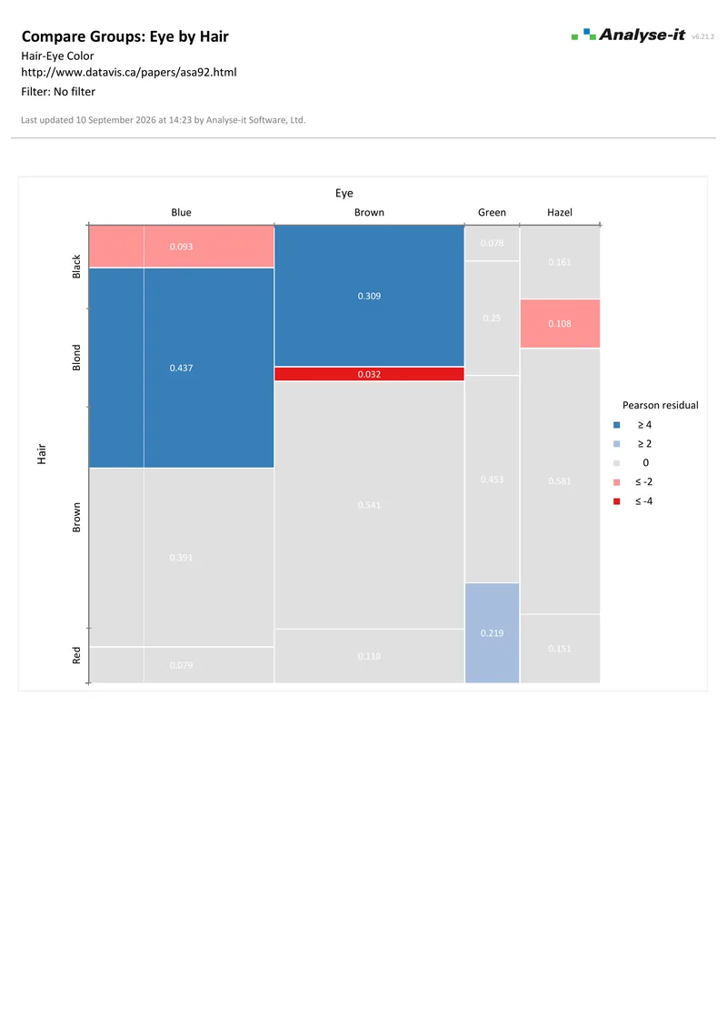
Hair and eye colour, 4×4 table.
592 observations. Clustered frequency plot of the conditional proportions, Pearson χ² test for independence and a mosaic plot. Standard
Related contingency table report 1 page Related contingency table
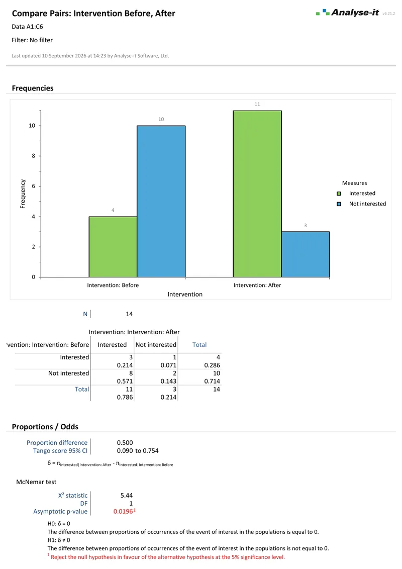
Before and after an intervention, 2×2 table.
14 paired observations. Clustered frequency plot, proportion difference with a Tango score 95% CI and the McNemar test of marginal homogeneity. Standard
One-way ANOVA report 5 pages One-way ANOVA, two ways
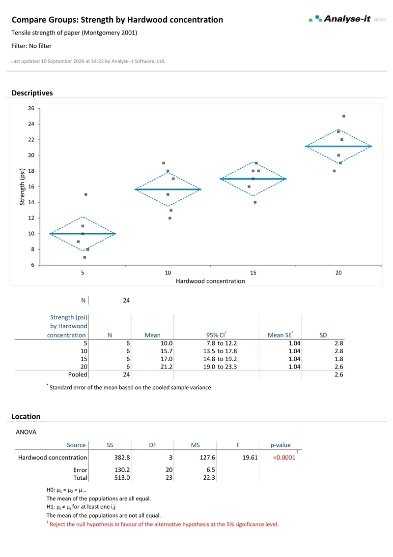
Tensile strength of paper by hardwood concentration.
Montgomery 2001. Four groups of six observations, analysed through both Compare Groups and Fit Model so the two routes can be compared. Dot plots with confidence diamonds, ANOVA, Tukey-Kramer over six contrasts and a Mean-Mean scatter plot. Standard
Two-way ANOVA report 3 pages Two-way ANOVA
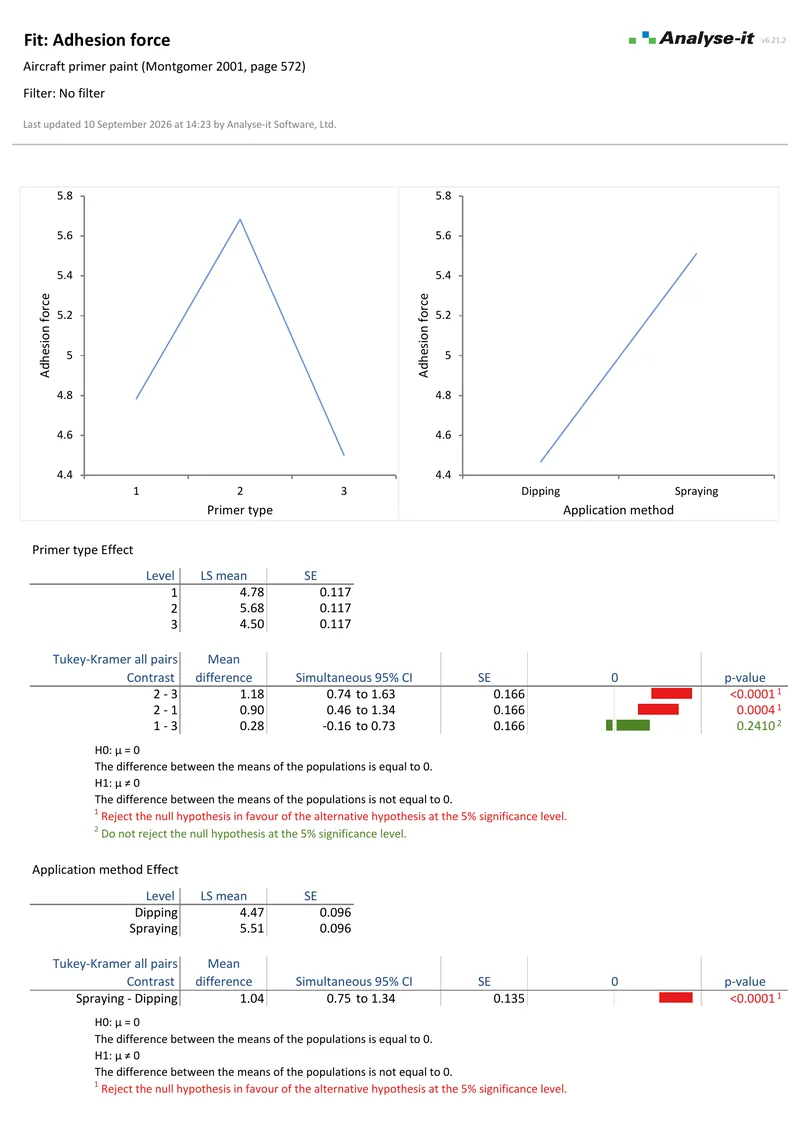
Aircraft primer paint adhesion force.
Montgomery 2001, page 572. Three primer types × two application methods, 18 observations, R² = 0.908. F tests for each term — both main effects significant, the interaction not — LS means, main effect plots and Tukey-Kramer on both factors. Standard
Three-factor ANOVA report 3 pages Three-factor ANOVA
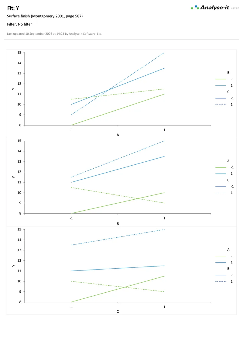
Surface finish, 2³ factorial design.
Montgomery 2001, page 587. 16 observations with every two-way and three-way interaction fitted. Only factor A is significant at 5%. Main effect plots and interaction effect plots. Standard
ANCOVA report 2 pages ANCOVA
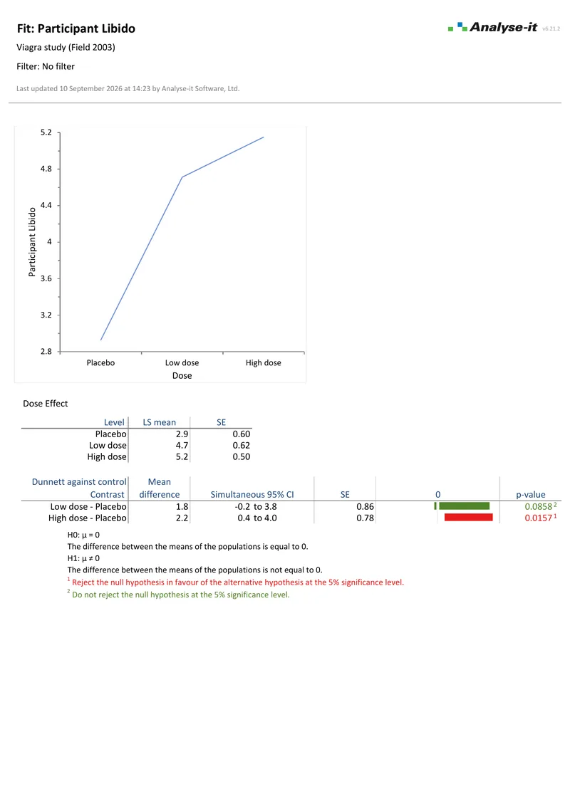
Three dose levels with a covariate, 30 participants.
Field 2003. A three-level factor — placebo, low dose, high dose — with a participant-level covariate, 30 observations. F tests for dose and covariate, LS means, main effect plot and Dunnett comparisons against the placebo control. Standard

Regression and multivariate

Fitting a model to explain or predict a response, and reducing many correlated variables to a few. 6 examples

Power regression report 4 pages Simple regression, power fit
TV advertising budget against retained impressions.
21 observations. Power function fit with a 95% confidence band, R², AIC, AICc and BIC, parameter estimates with CIs, correlation and covariance of the estimates, residual plot, normality diagnostics and an outlier, leverage and influence plot. Standard
Multiple regression report 4 pages Multiple regression
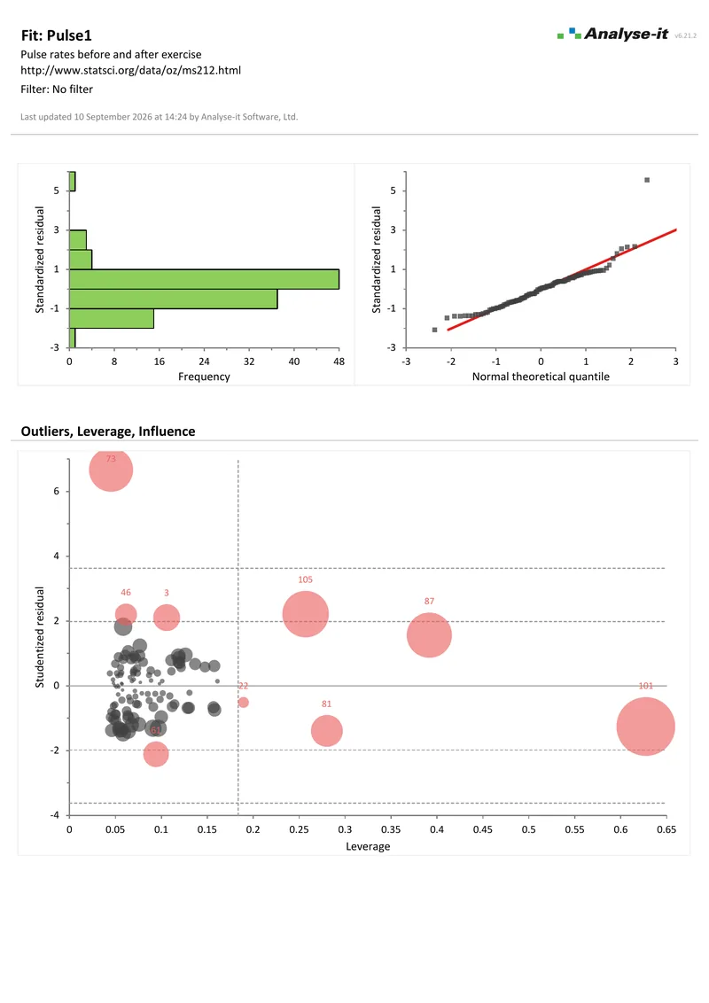
Pulse rates before and after exercise, 8 predictors.
109 observations, three continuous predictors and five categorical. Parameter estimates with 95% CIs and VIF, F tests for each term, leverage plots for every predictor, residual diagnostics and an outlier, leverage and influence plot. Standard
Logistic regression report 2 pages Binary logistic regression
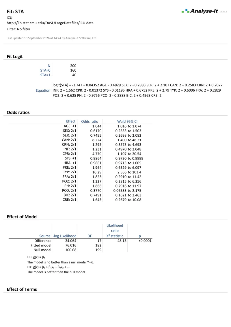
Intensive care unit survival, 17 predictors.
200 observations. Odds ratios with Wald 95% CIs and likelihood ratio tests for the model and for each term. Age, cancer, CPR, systolic blood pressure and admission type are significant at 5%. Standard
Simple logistic regression report 2 pages Simple logistic regression
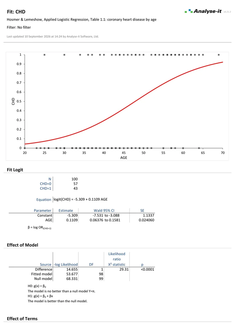
Coronary heart disease by age.
Hosmer and Lemeshow, table 1.1. 100 observations and a single continuous predictor. Fitted logit with parameter estimates and Wald 95% CIs, the odds ratio per year of age and a likelihood ratio test for the model. Standard
Correlation matrix report 2 pages Correlation matrix
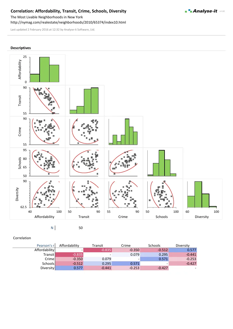
New York neighbourhood liveability, 5 variables.
50 observations. Pearson r matrix with a colour map, a scatter plot matrix and every pairwise coefficient with a 95% CI and a significance test. Standard
Principal component analysis report 3 pages PCA and factor analysis
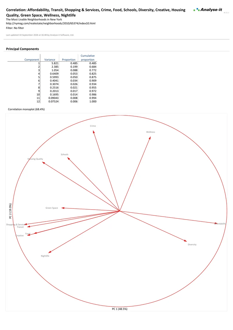
New York neighbourhood liveability, 12 variables.
50 neighbourhoods. Principal components with eigenvalues and coefficients and a biplot labelled by borough, a correlation monoplot and a common factor analysis reporting uniqueness, communality and factor loadings. Two components carry 68.4% of the variance. Standard

Survival analysis

Time to an event, with censored observations kept in the analysis rather than thrown away. 2 examples
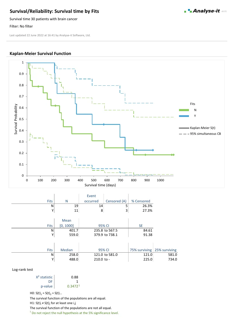
Kaplan-Meier survival report 3 pages Kaplan-Meier survival
Brain cancer survival, 30 patients.
Two analyses of one dataset — survival by treatment, 19 patients against 11 and survival by tumour grade over three groups. Survival curves with confidence bands, mean and median survival with CIs, quartile survival times and a log-rank test for each. Medical
Cox proportional hazards report 2 pages Cox proportional hazards
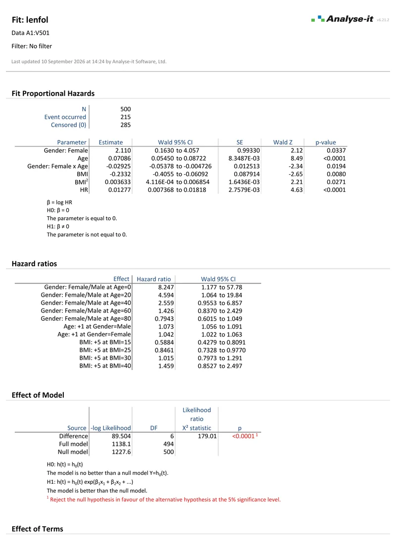
Worcester Heart Attack Study, 500 patients.
215 events and 285 censored. Sex, age, their interaction, body mass index as a quadratic and heart rate. Parameter estimates with Wald 95% CIs, hazard ratios evaluated at several ages and BMI values and likelihood ratio tests for the model and each term. Medical