Contingency table analysis with mosaic plots Chi-square, Fisher exact, McNemar, proportion difference and ratio tests, odds ratios with multiple CI methods and mosaic plots with residual colouring — for independent and related tables.

Every feature from all five editions for 15 days.
Standard edition from US$ 155 a year · 30-day money-back guarantee.
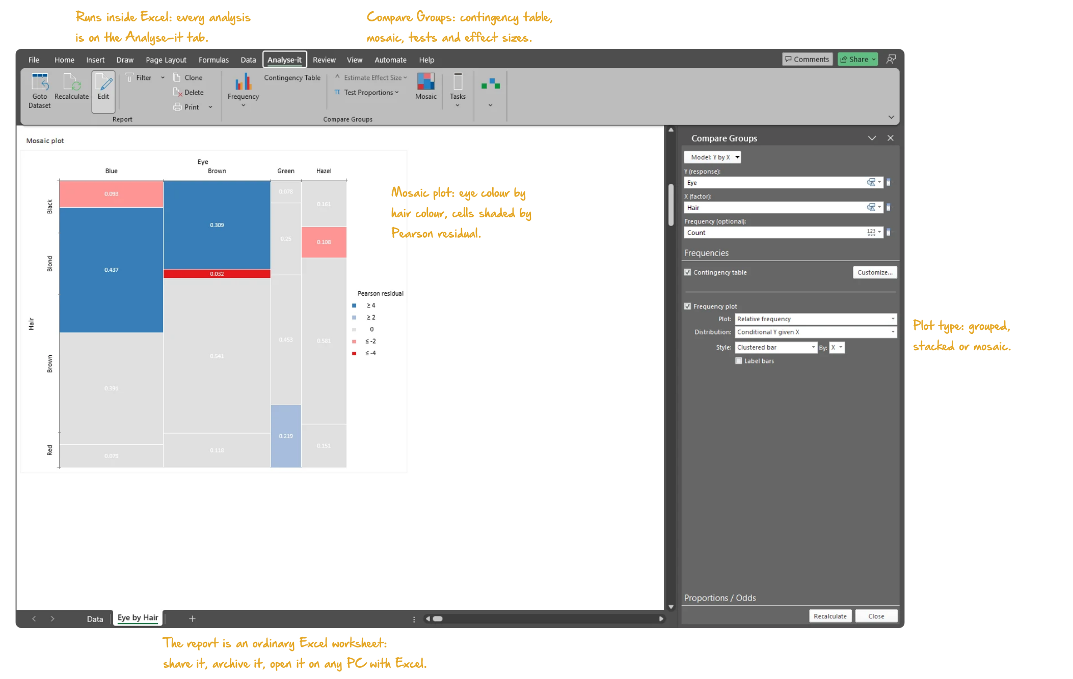
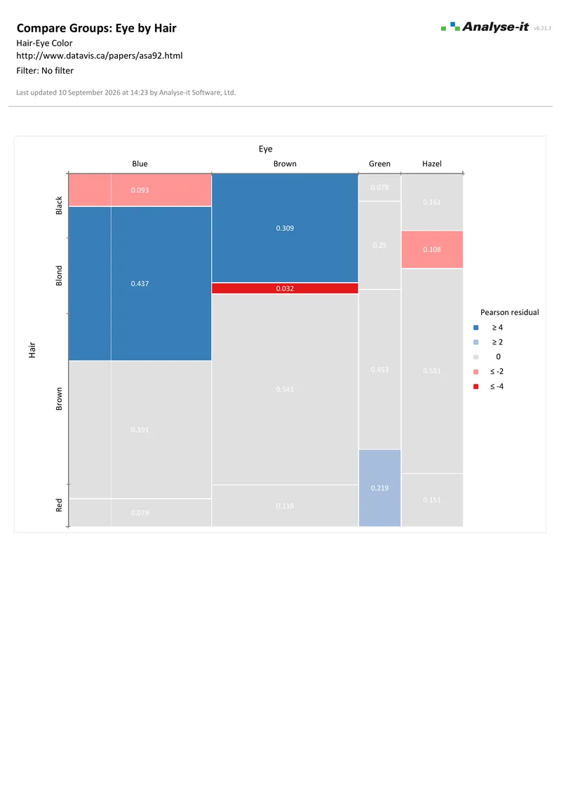
Microsoft Excel with the Analyse-it tab selected, showing the contingency table report for hair and eye colour: the mosaic plot with each tile coloured by its Pearson residual and the residual colour scale beside it, and the Compare Groups task pane open. Handwritten notes: Runs inside Excel: every analysis is on the Analyse-it tab; Compare Groups: contingency table, mosaic, tests and effect sizes; Mosaic plot: eye colour by hair colour, cells shaded by Pearson residual; Plot type: grouped, stacked or mosaic; The report is an ordinary Excel worksheet: share it, archive it, open it on any PC with Excel.

Categorical data analysis beyond the χ² test

Excel’s built-in CHISQ.TEST returns a p-value for a table whose expected frequencies you have already worked out, and stops. No mosaic plot to see where the association lies. No risk difference or odds ratio with a score confidence interval. No distinction between independent and related tables, and no McNemar test for before-and-after designs. When the data are categorical — pass/fail, treated/untreated, exposed/unexposed — you need tests designed for proportions, not means, and knowing that two variables are associated is rarely enough.

Where is the association strongest? How large is the effect — as an absolute difference, a relative risk or an odds ratio? Is the confidence interval precise enough to act on? And when the same subjects are measured twice, which test applies?

Contingency table, grouped and stacked frequency plots

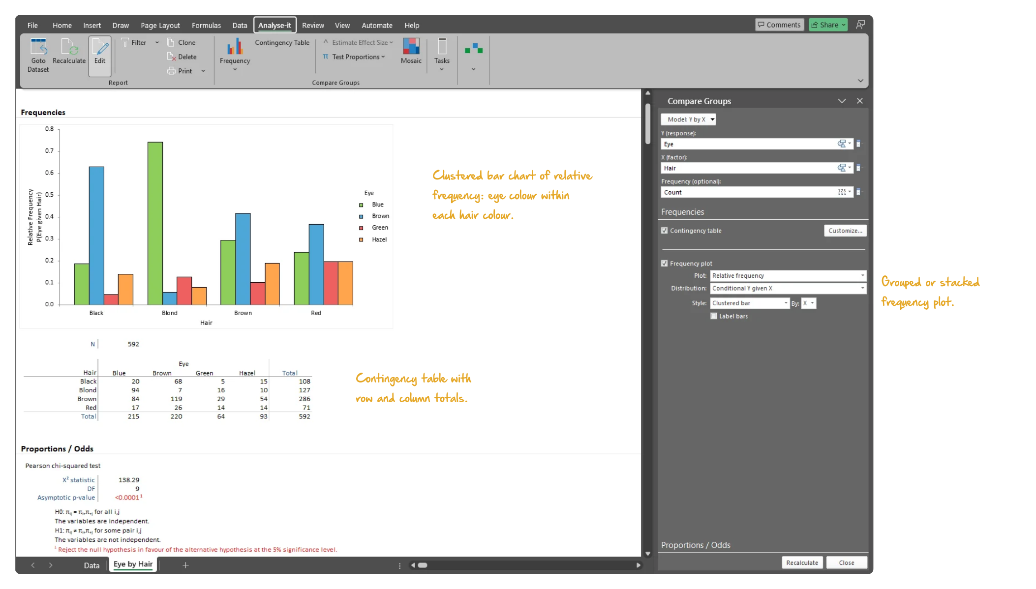
See the table and the conditional proportions before any test. The contingency table shows the counts for every combination of the two variables, with the marginal totals. Grouped and stacked frequency plots show the proportion of each category within each group, so a difference between the groups is visible before it is tested.
  • Contingency table
  • Row, column and total percentages; joint and conditional distributions
  • Expected frequencies and Pearson residuals
  • Grouped frequency plot
  • Stacked frequency plot
Microsoft Excel showing the Frequencies section of the hair and eye colour report: the grouped frequency plot of the relative frequency of each eye colour within each hair colour, the count of 592 observations, and the 4 by 4 contingency table with row and column totals, with the task pane open. Handwritten notes: Clustered bar chart of relative frequency: eye colour within each hair colour; Contingency table with row and column totals; Grouped or stacked frequency plot.
Hair and eye colour in a 4×4 table: the grouped frequency plot of eye colour within each hair colour, and the contingency table with its marginal totals.

Pearson χ² and likelihood ratio G² tests, with the mosaic plot

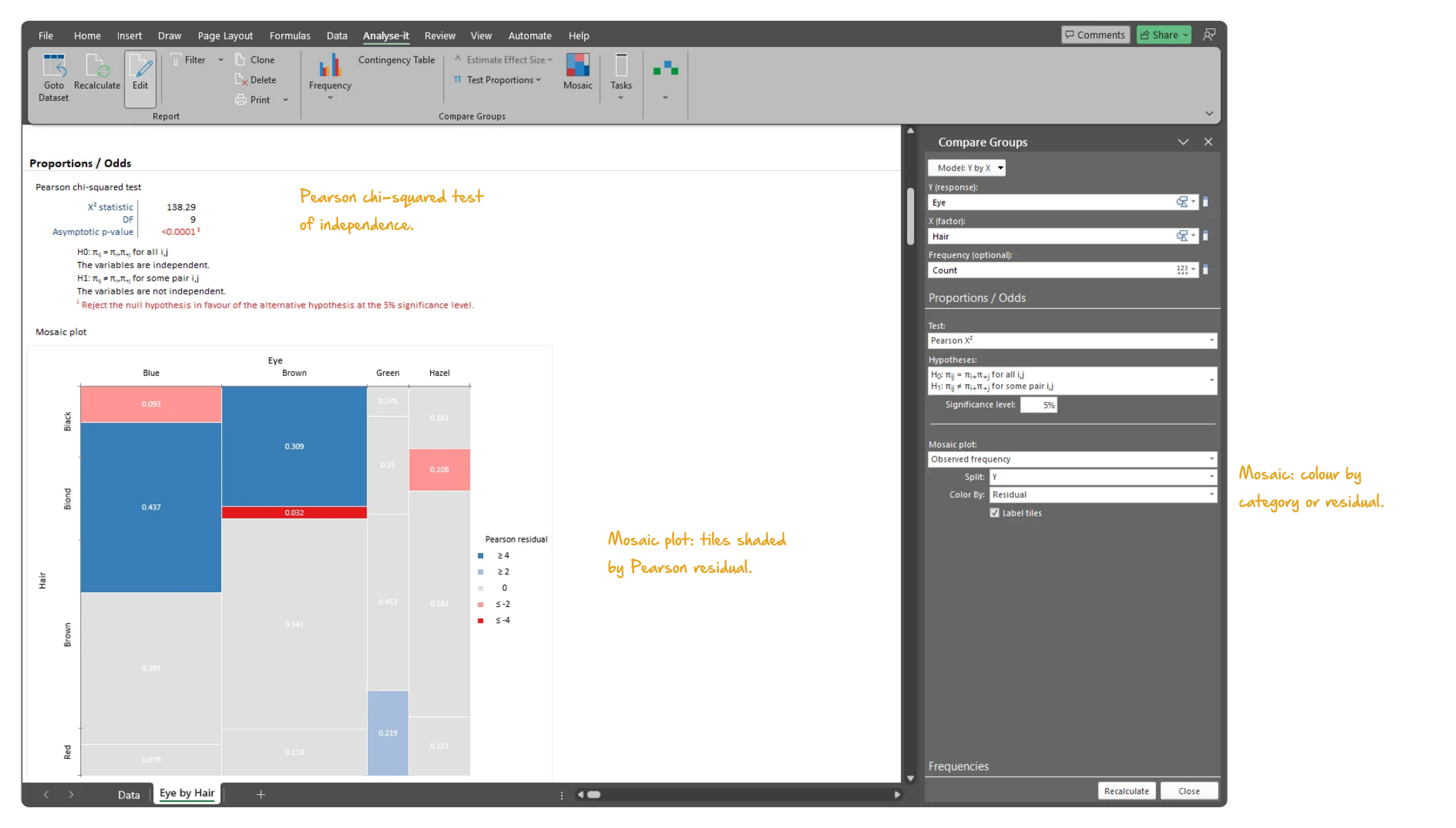
Pearson χ² and likelihood ratio G² tests tell you whether two categorical variables are associated. The mosaic plot shows where. Each tile’s area represents the proportion, and colouring by Pearson residual highlights the cells that depart most from what independence would predict.
  • Pearson χ² test for independence / equality of proportions
  • Likelihood ratio G² test for independence
  • Mosaic plot coloured by category or Pearson residual
Microsoft Excel showing the Proportions / Odds section of the hair and eye colour report: the Pearson chi-squared test table with the statistic, degrees of freedom, p-value and the null and alternative hypotheses, and the mosaic plot beneath it coloured by Pearson residual, with the task pane open. Handwritten notes: Pearson chi-squared test of independence; Mosaic plot: tiles shaded by Pearson residual; Mosaic: colour by category or residual.
The Pearson χ² test for independence of hair and eye colour, and the mosaic plot beneath it with each tile coloured by its Pearson residual.

Fisher exact test, risk difference, risk ratio and odds ratio in 2×2 tables

A significant χ² test does not tell you how large the effect is. For a 2×2 table of independent observations, Fisher’s exact test tests for independence and the score Z test for a difference between the two proportions. Proportion difference (risk difference), proportion ratio (risk ratio) and odds ratio each answer a different question — absolute difference, relative risk or odds. Each has score-based or exact confidence intervals that perform well even with small samples or proportions near 0 or 1.

  • Fisher exact test for independence
  • Score Z test for difference between proportions
  • Proportion difference (risk difference) with Miettinen-Nurminen score or Newcombe score CI
  • Proportion ratio (risk ratio) with Miettinen-Nurminen score CI
  • Odds ratio with hypergeometric exact or Miettinen-Nurminen score CI

McNemar exact test, Tango score CI and odds ratio for 2×2 related tables

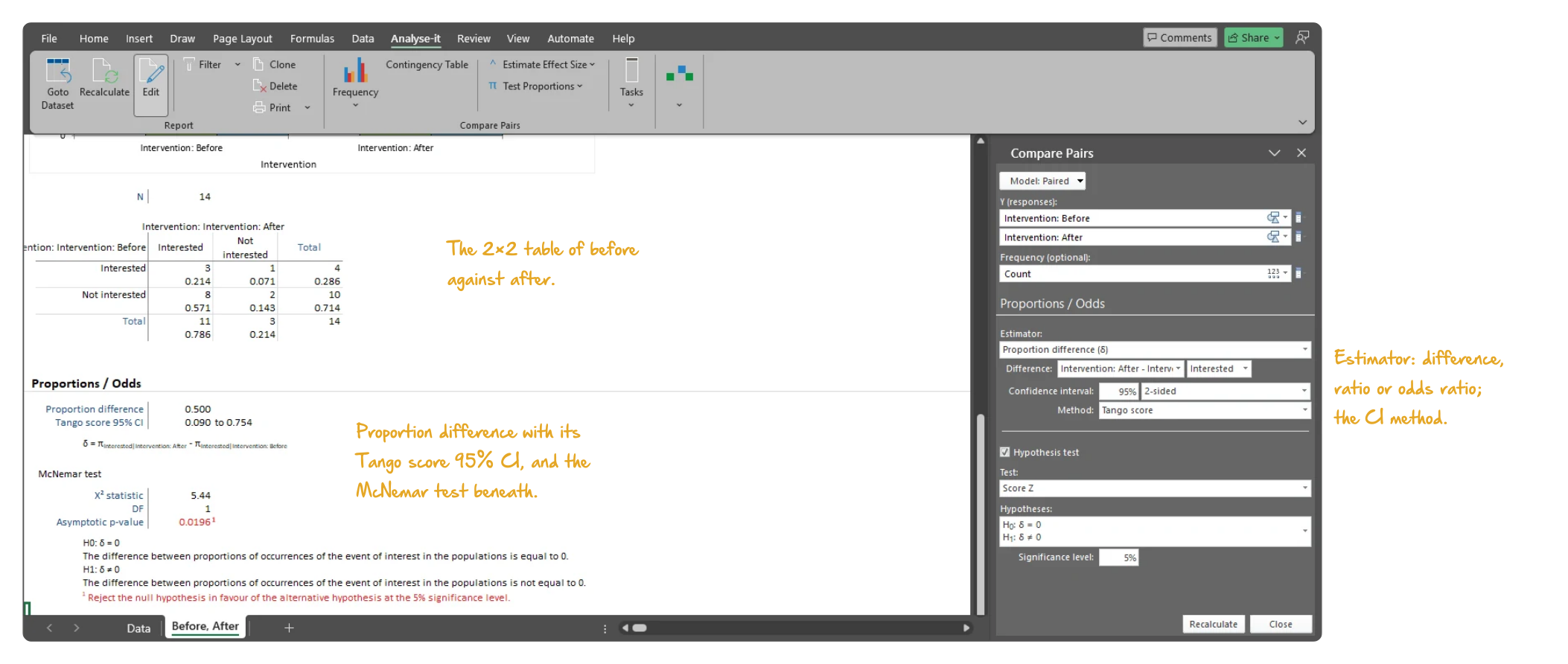
When the same subjects are measured twice, the observations are paired and the standard χ² test does not apply. Before and after treatment, or two raters classifying the same cases, are the usual designs. The McNemar-Mosteller exact test for marginal homogeneity handles the dependent structure correctly. So do the proportion difference with a Tango score CI and the odds ratio with an exact or Wilson score CI.
  • McNemar-Mosteller exact test for symmetry / marginal homogeneity
  • Score Z test for difference between proportions
  • Proportion difference with Newcombe score or Tango score CI
  • Odds ratio with binomial exact or Wilson score CI
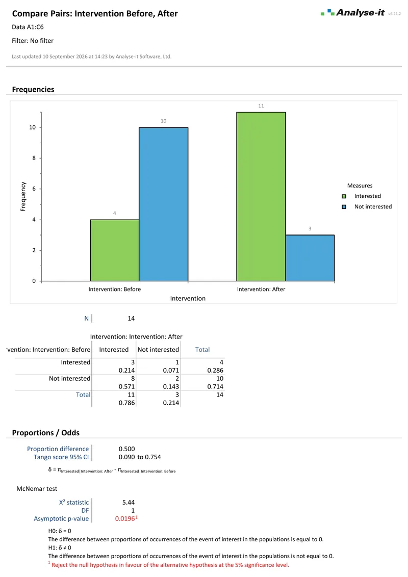
Microsoft Excel showing the related-table report for interest before and after an intervention: the 2 by 2 contingency table with counts, proportions and marginal totals, the proportion difference with its Tango score 95% confidence interval, and the McNemar test with its hypotheses, with the Compare Pairs task pane open. Handwritten notes: The 2×2 table of before against after; Proportion difference with its Tango score 95% CI, and the McNemar test beneath; Estimator: difference, ratio or odds ratio; the CI method.
A 2×2 related table of interest before and after an intervention: the proportion difference with its Tango score 95% CI, and the McNemar test for marginal homogeneity.

Example analyses

See contingency table results in detail — independence tests, mosaic plots, proportion tests and effect sizes with CIs.

Contingency Tables 1 p2 2 pages Independent contingency table
Hair and eye colour, 4×4 table.
592 observations. Clustered frequency plot of the conditional proportions, Pearson χ² test for independence and a mosaic plot.
Contingency Tables 2 1 page Related contingency table
Before and after an intervention, 2×2 table.
14 paired observations. Clustered frequency plot, proportion difference with a Tango score 95% CI and the McNemar test of marginal homogeneity.

Part of the Standard edition

Contingency table analysis is one part of a complete statistical analysis toolkit. The Standard edition also includes ANOVA and ANCOVA, simple and multiple regression, logistic regression, PCA and factor analysis, descriptive statistics, hypothesis testing and correlation. See everything in the Standard edition →

Learn how the study design determines the procedure: chi-square, Fisher exact or McNemar? Then see Cohen’s kappa and weighted kappa when the question is agreement rather than association.

Software you can trust

Validated calculations Every statistic tested against the NIST Statistical Reference Datasets, published datasets and thousands of internal test cases. No reliance on Excel’s built-in functions. How Analyse-it is developed and validated →
Data stays on your PC No cloud processing, no uploads, no third-party access. Your data never leaves your computer — essential when working with sensitive, confidential or patient-identifiable data.
Standard Excel workbooks Analyses are ordinary Excel workbooks that you can share with colleagues, archive for audit and open on any machine with Excel — no Analyse-it licence required.
No formulas to break Results contain no formulas, so there is nothing to overwrite and no cell reference to break. The results you reported will be exactly what you find when you reopen the workbook.

Free trial and pricing

Try it on your own data first. The 15-day trial is every feature from all five editions — install it and start straight away.

Standard edition: US$ 155 per year or US$ 395 for a perpetual licence. Every purchase carries a 30-day money-back guarantee. Need a quote for purchasing? Add the licence to the cart and save it as a PDF quote.