Learn how to estimate the precision of a measurement procedure for product performance characteristics, for FDA 510k submissions and product marketing.
In this tutorial you will use the CLSI EP05-A3 procedure to establish the precision.
Estimate the precision of the measurement procedure at a single site.
The variability plots show a simple visual assessment of the closeness of agreement between the measured quantity values. The purple lines show the mean of each run, the light blue lines show the mean of each day, and the dark blue line the overall grand mean.
The abbreviated variance components table shows the required precision statistics expressed numerically as the standard deviation (SD) and coefficient of variation (CV).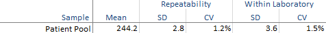
The detailed variance components table show the precision expressed numerically as the chosen measure of imprecision along with a confidence interval for each component. 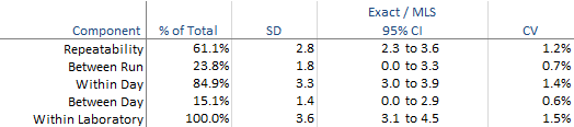
Estimate the precision of the measurement procedure at multiple sites and samples.
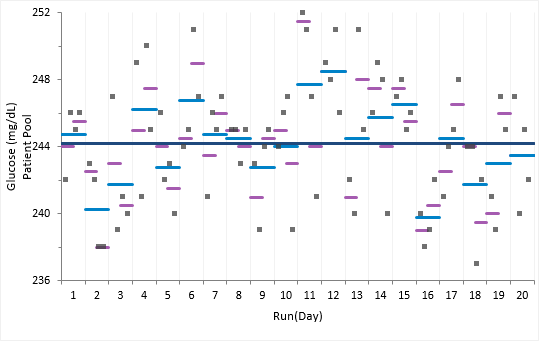
The variability plots show a simple visual assessment of the closeness of agreement between the measured quantity values. The purple lines show the mean of each run, the light blue lines show the mean of each laboratory, and the dark blue line the overall grand mean.
You should observe the scatter of the points to ensure there are no obvious problems. No individual measurements stand out as highly aberrant relative to the bulk of the data and none of the plots exhibit any apparent drift capable of distorting the results.
The abbreviated variance components table shows the required precision statistics expressed numerically as the standard deviation (SD) and coefficient of variation (CV).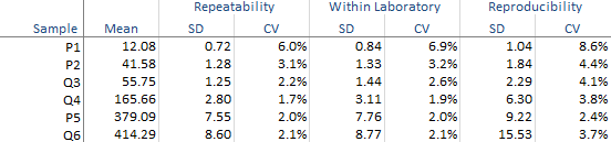
The detailed variance components table show the precision expressed numerically as the chosen measure of imprecision along with a confidence interval for each component.
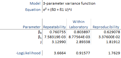
Fit a precision profile function to describe the imprecision across the measuring interval.
The precision profile show the relationship between the imprecision and the measurand level. The variance function fit describes the relationship as a continuous function.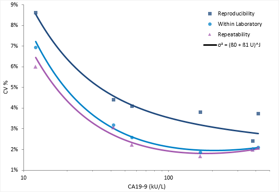
The variance function describes the relationship between the variance and concentration using a 3-parameter power model typically used for immunoassays.