
A reference interval is defined by its 2.5th and 97.5th percentiles, so the estimate comes from the tails of the distribution. The tails are also where two common features of reference data do the most harm.
A single erroneous extreme value can drag a limit noticeably. An untreated skew can put a limit in the wrong place altogether. Screening for outliers and handling the distribution’s shape are therefore not preliminary steps to complete before the real analysis. Together, the two steps largely are the analysis.
Reference samples come from apparently healthy volunteers, but errors occur: a transcription slip, a mislabelled tube, or an individual who was not as healthy as assumed. Outlier screening finds candidates for these.
But a value being extreme is not proof it is wrong. Some genuinely healthy people sit at the edges of a distribution. Deleting them because they are inconvenient narrows the interval artificially. The right approach is to flag extreme values, investigate for a cause, and remove only those with a justified reason. Do not trim the tails simply to make the interval look neat.
EP28-A3c points to outlier rules designed for this setting rather than a generic one. Tukey’s fences flag values beyond a multiple of the interquartile range. The fences are robust because the quartiles are not themselves distorted by the extremes being tested. Rules of the Dixon and Reed type judge a candidate by its distance from its neighbours relative to the overall range.
Masking is the trap to avoid: a rule that uses the mean and SD to find outliers is undermined by the very outliers it is looking for. Tukey’s fences resist masking. Dixon’s gap rule does not, because two outliers side by side hide each other, so use it only where a single outlier is plausible. Apply the screen on the appropriate scale too, after any transformation rather than before it. A value that looks extreme on a skewed raw scale may be unremarkable once the skew is removed.
Reference distributions are frequently right-skewed, with a long upper tail. Skew matters because the parametric method, which computes the limits from the mean and SD, assumes a Gaussian shape.
Applied to untransformed skewed data, the parametric method puts the limits in the wrong place: the upper limit too low, the lower limit implausibly low or negative. Confirm the shape first rather than assuming normality. Use a normal Q-Q plot together with a formal test such as Shapiro–Wilk or Anderson–Darling.
Two sound routes handle skew. The first is to transform the data to normality, then apply the parametric method on the transformed scale and back-transform the limits. A logarithm often suffices, or a Box–Cox or one of the other transformations chosen to fit. The second is to sidestep the assumption with the non-parametric method, which makes no claim about the distribution’s shape. The robust method assumes symmetry, so a skewed sample still needs transforming first.
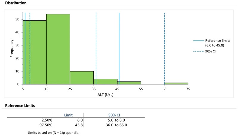
The transformation route keeps the efficiency of the parametric method when it works. The non-parametric route is simpler when the skew is awkward and you have at least 120 individuals. With fewer, transform and use the parametric or robust method. The worked example below log-transforms a skewed ALT dataset and estimates non-parametric limits. The transformation leaves non-parametric limits essentially unchanged, because they depend only on the rank order of the data. What it changes is the outlier screen, which then runs on a near-symmetric scale.
Download the CLSI EP28-A3c example workbook (.xlsx): ALT reference intervals by sex, 120 observations each, log-transformed and screened with an outlier box plot, with non-parametric limits and 90% confidence intervals. The workbook is ready to open in the Analyse-it trial.
The example workbook is downloading.
It opens in Excel on its own — the data and the finished results are both in it. Analyse-it is what lets you change the analysis and re-run it, try the same study on your own data, or work through it to see how the software handles it.
Every feature from all five editions for 15 days.
Deleting extreme values because they are inconvenient. Some healthy people sit in the tails. Remove outliers only with a justified cause, not to tidy the interval.
Using a mean-and-SD outlier rule. The outliers distort the very statistics used to find them. Prefer Tukey’s quartile-based fences, which resist masking.
Applying the parametric method to skewed data. The method assumes normality, so untransformed skew puts the limits in the wrong place. Transform first, or use the non-parametric method if you have 120 or more individuals.
Screening on the wrong scale. A value extreme on a skewed raw scale may be ordinary once transformed. Screen after transformation, not before.
Analyse-it does the screening before the estimate, on your own reference data, inside Excel:
Every feature from all five editions for 15 days. Reference intervals are in the Medical, Method Validation and Ultimate editions, from US$ 340 a year. Validated against NIST and CLSI reference datasets. See choosing a reference interval method.