Choosing a reference interval method Parametric, non-parametric, robust, bootstrap, or Harrell–Davis? Which quantile method to use depends on how many reference individuals you have and how their values are distributed. A decision guide following CLSI EP28-A3C.

A reference interval, often called the reference range or loosely the normal range, is the central 95% of results from a suitable reference population. A clinician reads a patient’s result against it to decide whether the result is unremarkable or worth acting on. Two reference limits bound it: the 2.5th and 97.5th percentiles of the reference distribution.

Estimating those two percentiles sounds simple. CLSI EP28-A3C offers several ways to do it. They are not interchangeable. The right choice depends on two questions: how many reference individuals you have, and whether their values follow a Gaussian distribution. Get the pairing wrong and you either throw away information or report limits your data cannot support.

The sample-size question comes first

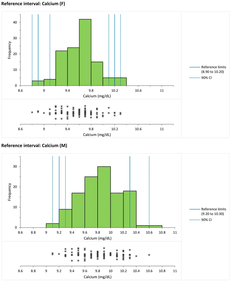
EP28-A3C sets 120 reference individuals per partition as the threshold for the recommended non-parametric method. That number is not arbitrary. One hundred and twenty is roughly the smallest sample that lets you estimate the 2.5th and 97.5th percentiles directly, with 90% confidence intervals on each limit, and without leaning on a distributional assumption.

Below 120 you have not failed. You have simply changed which methods are appropriate. With fewer individuals the non-parametric estimate becomes unstable in the tails, and you move to a parametric or robust approach that extracts more from a smaller sample by making (and checking) an assumption. Do not report a bare non-parametric interval from 40 samples as though it carried the same weight as one from 120.

The methods, and what each assumes

Non-parametric quantile is the EP28 default at n ≥ 120. It ranks the data and reads the percentiles off directly, assuming nothing about the shape of the distribution. The method is robust and simple, but it needs that large sample, and its confidence intervals on the limits are wide. Analyse-it offers three standard computation approaches, (N+1)p, Np+½, and (N+⅓)p+⅓, which differ only trivially at realistic sample sizes.

Parametric quantile assumes the values are Gaussian, if necessary after a transformation, and computes the limits from the mean and SD. Where that assumption holds, the parametric method is markedly more efficient than the non-parametric one: it works at smaller sample sizes and gives tighter confidence intervals. Where the assumption does not hold, and the data were not transformed to normality first, the limits are simply wrong. That is why the normality check and the transformation step matter.

Robust (bi-weight) is EP28’s small-sample option, workable with as few as around 20 reference individuals. It estimates the limits iteratively, down-weighting values far from the centre. That makes it resistant to the occasional outlier a small sample cannot absorb without distortion. The robust method is the pragmatic choice when recruiting 120 healthy individuals per partition is not realistic, and for a partitioned analyte it often is not.

Harrell–Davis estimates each quantile as a weighted combination of all the order statistics rather than one or two ranked values. That lowers the variance of the estimate and behaves better in the tails, which is exactly where reference limits live. Harrell–Davis is a strong choice at moderate sample sizes, when you want more efficiency than the simple non-parametric method without committing to normality.

Bootstrap resamples the data to build confidence intervals on the limits without a distributional assumption. Bootstrapping is most useful when the analytic confidence intervals are questionable, or when you want a distribution-free interval on a limit estimated by another method.

A decision guide

Before you commit to a method, do two things. Screen for outliers with a Tukey box plot. Then check normality, using Shapiro–Wilk or Anderson–Darling together with a normal Q-Q plot. After that:

Situation	Method
n ≥ 120, distribution non-Gaussian or unknown	Non-parametric quantile — the EP28 default
n ≥ 120, distribution Gaussian or transformable to Gaussian	Parametric — tighter CIs, once normality is confirmed
n below 120 (down to ~20), more individuals not obtainable	Robust bi-weight
Moderate n, want efficiency and good tail behaviour without assuming normality	Harrell–Davis
Analytic CIs doubtful, or you want distribution-free CIs on a limit	Bootstrap
Adopting an interval established elsewhere	Transfer and verify — see below

A skewed distribution does not force you onto the non-parametric method. If the skew is transformable, normalise the data first, estimate the limits parametrically, and back-transform them to the original scale. The transformations available for this are log, square root, cube root, reciprocal, Box-Cox, Manly exponential, and two-stage exponential or modulus.

Partitioning: when one interval is not enough

Many analytes need separate intervals for subgroups. Alkaline phosphatase by sex and age group is the classic example. Partition when the subgroups differ enough that a combined interval would misclassify results at the margins. The complication is arithmetic. Each partition needs its own adequate sample. Two sex partitions at the non-parametric threshold means 240 individuals, not 120. That is often why a careful lab uses the robust or parametric methods for each partition.

Transferring and verifying an existing interval

You do not always have to establish an interval from scratch. EP28-A3C allows you to transfer an interval, from a manufacturer, a published study, or another method via a method-comparison regression, and verify that it holds in your population with a small study, typically around 20 reference individuals per partition.

If no more than a small proportion of those fall outside the transferred interval, a binomial test confirms the interval is acceptable for your use. Verification is a fraction of the work of establishment, and for most laboratories adopting a well-characterised assay it is the right route. The mercury transfer example below walks through one.

Downloads

A worked example for each approach, ready to open in the Analyse-it trial:

• Non-parametric, partitioned — calcium, partitioned by sex (the histogram above).
• Transformation — ALT, a skewed analyte with outlier screening, normalised then estimated on the transformed scale.
• Transfer and verify — mercury, an existing interval transferred and verified against a small sample.
• Robust bi-weight — calcium, the small-sample robust method.

Common mistakes

Reporting a non-parametric interval from too small a sample. Below 120 the tails are unstable. The number you print will not be reproducible. Move to a robust or parametric method rather than pretending the sample is larger than it is.

Applying the parametric method without checking normality. The efficiency of the parametric approach is real, but it is conditional. An untested normality assumption on a skewed analyte produces limits that are confidently wrong. Check first. Transform if needed.

Ignoring the confidence intervals on the limits. A reference limit is an estimate with uncertainty, and at realistic sample sizes that uncertainty is not small. Quoting the limits without their confidence intervals hides how much room there is around them.

Partitioning without the sample to support it. Splitting by sex and age is right in principle but doubles or quadruples the sample you need. Partition deliberately, and match the method to the sample each partition actually has.

Establishing when you could verify. If a robust interval already exists for your method, a 20-sample verification may be all you need. Recruiting 120 individuals to re-establish it from scratch is effort spent where a transfer would have done.