Every feature from all five editions for 15 days.
Method Validation edition from US$ 475 a year · 30-day money-back guarantee.
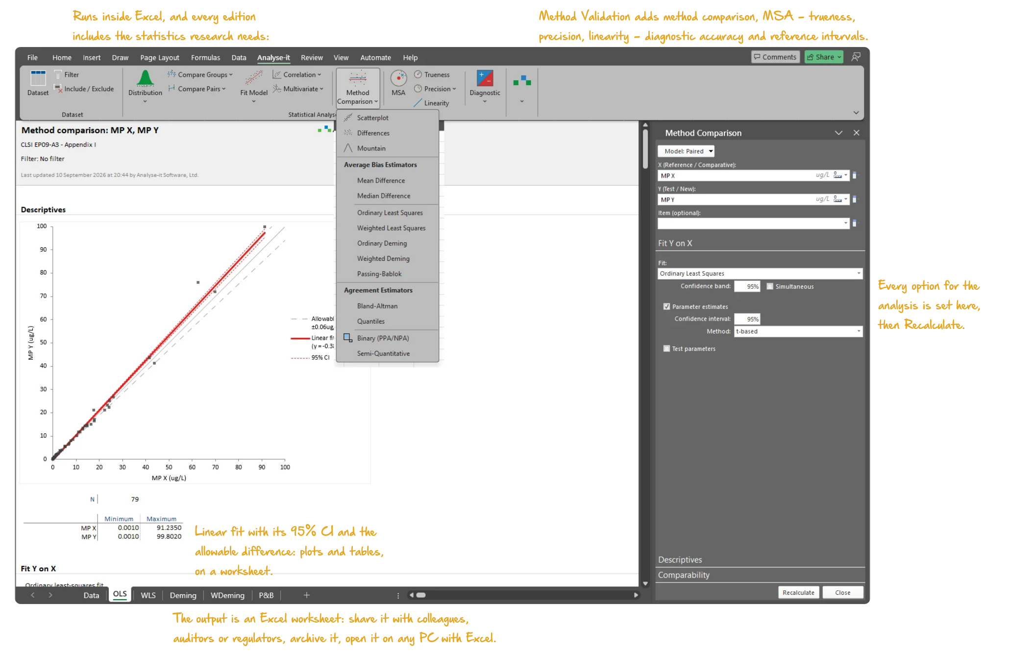
A method validation under ICH Q2(R2) and an accreditation exercise under ISO/IEC 17025 ask for the same evidence in different words. The method must measure what you think it measures, over the range you claim, with a scatter and a bias you have quantified rather than assumed. The same must still be true months later.
The statistics behind that evidence are not exotic. What makes it slow is that each characteristic ends up in a different tool. The calibration curve sits in one spreadsheet, the intermediate precision in a statistics package somebody in the group knows, the robustness study in a table nobody quite trusts. Analyse-it runs all of it inside Excel, so the raw data, the analysis and the report that goes into the validation file are one workbook. The workbook is reviewable, archivable and reopenable years later.



ICH Q2(R2) names the characteristics; ISO/IEC 17025 asks you to validate to the extent the application requires. Either way these are the studies, with a guide to designing each one and setting its acceptance criterion. Treat the table as a map rather than a sequence. The regression, variance components and interval estimates underneath are all available on their own, for development and troubleshooting work that no validation document covers.
| Characteristic | The study | Guide |
|---|---|---|
| Specificity & selectivity | Recovery against an allowable bias, with interference by experimental design | Interference and recovery |
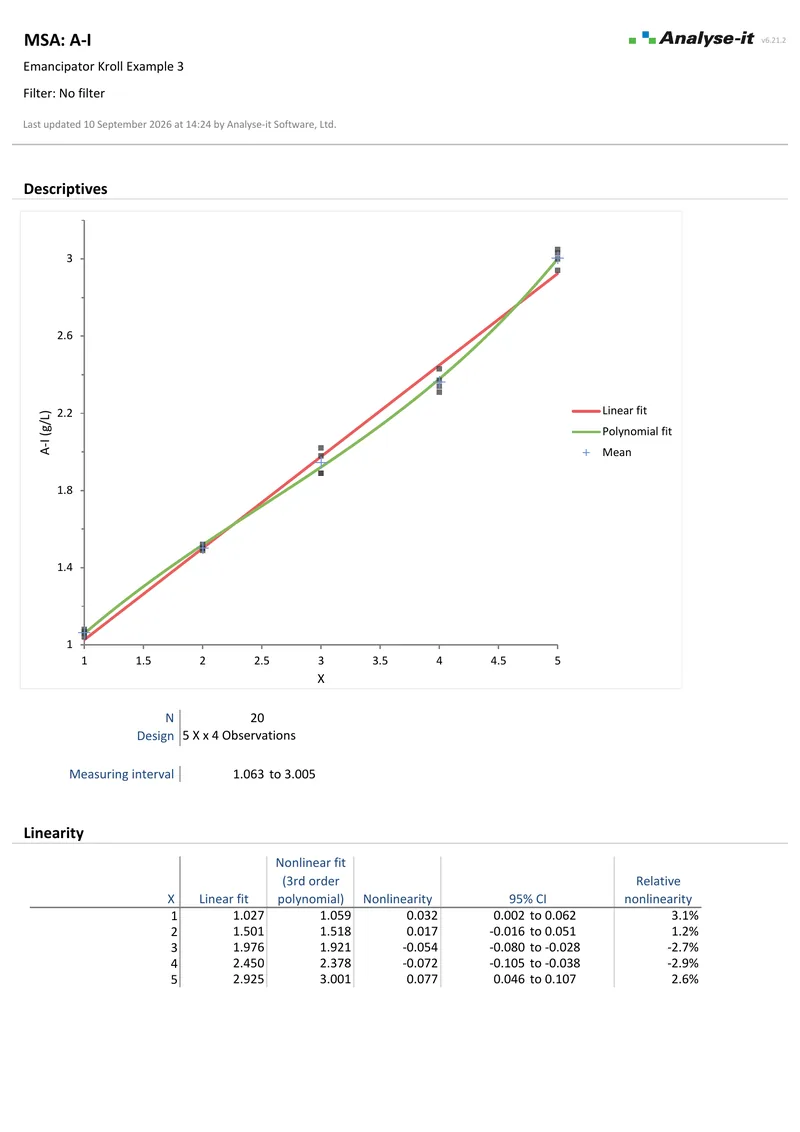
| Linearity & range | Regression across the claimed range with residual diagnostics and a nonlinearity test | Assessing linearity |
| The calibration model | Model choice and weighting, checked by using the curve backwards | Fitting a calibration curve |
| Accuracy — trueness | Recovery against a reference material or comparative method, with a confidence interval on the bias | Trueness, precision and accuracy |
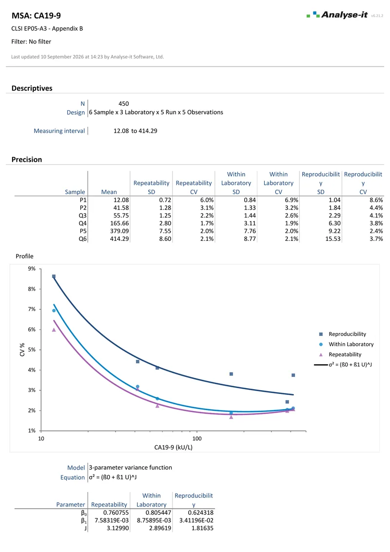
| Repeatability & intermediate precision | Nested replication across days, analysts and instruments, broken into variance components | Precision components |
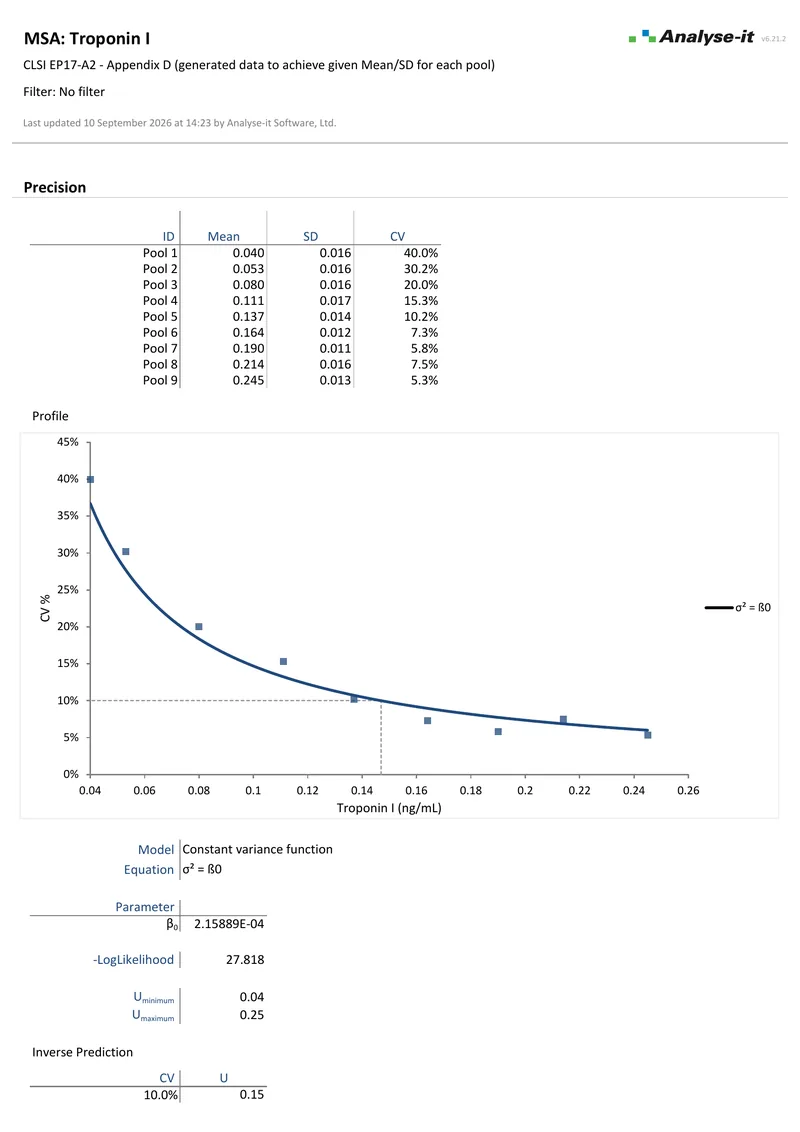
| Detection & quantitation limits | LoD from blanks and low-level samples; LoQ read off the fitted precision profile | LoQ from a precision profile |
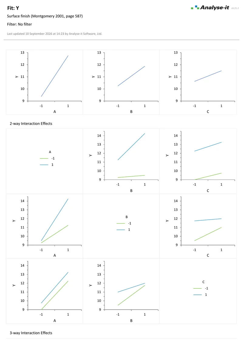
| Robustness (ICH Q14, development) | Factorial design varying the method parameters together, analysed as a multi-factor model | Robustness testing |
| Ongoing performance (ISO/IEC 17025) | Control charts on check standards and replicate controls | Which control chart |
| Measurement uncertainty (ISO/IEC 17025) | Built top-down from the precision and bias the validation already produced | Top-down uncertainty |
Method validation under ICH Q2(R2) covers the characteristics in order and what the 2023 revision changed. The guide also shows how the pharmaceutical vocabulary maps onto the clinical laboratory terms you will meet in the CLSI literature on the same statistics.
Running the method twenty times on one afternoon gives you repeatability and almost nothing else. Intermediate precision asks a different question — how much the result moves when the day, the analyst or the instrument changes. Answering it means a design where those factors are deliberately varied and then separated in the analysis. Pool them into one standard deviation and you cannot tell whether the variation you are seeing is worth investigating.
Analyse-it fits the nested design directly, including unbalanced ones where a second analyst ran fewer replicates. Each variance component is reported with a confidence interval rather than a bare estimate. That breakdown is what tells you whether tightening the method, retraining or recalibrating is the change worth making.
Precision and variance components →A high r² is the most over-trusted number in analytical chemistry. The value tells you the points are close to a line. What it does not say is whether the model is right at the bottom of the range, where the specification is usually tightest. Unweighted least squares fits the top of a wide calibration range at the expense of the low standards, which is exactly the wrong trade-off for a trace-level method.
Analyse-it fits linear, polynomial and linearisable models with the residual and influence diagnostics that show where the fit is failing. Weighted models are available in the linearity analysis, and curvature is tested explicitly rather than by eye. You can also set the interval you intend to report over separately from the interval you calibrated across. The two ranges are routinely, and expensively, confused. Analyse-it is not a 4PL or 5PL curve-fitting package. For a binding assay that needs one, use dedicated immunoassay software.
Linearity and measuring interval → Regression and model fitting →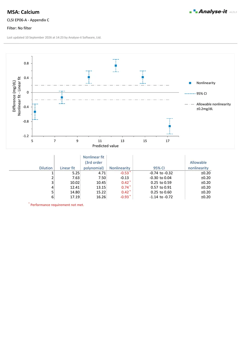 6 pages
EP06-A — Appendix C
6 pages
EP06-A — Appendix CA limit of quantitation quoted as “ten times the standard deviation of the blank” is a convention, not a measurement, and it is increasingly asked to justify itself. The defensible version defines the LoQ as the concentration at which imprecision first falls to a level you declared acceptable. That definition means fitting how imprecision changes across the range and reading the limit off that curve.
Analyse-it fits the precision profile and reads the LoQ from it. LoB and LoD are estimated by parametric, non-parametric or probit approaches, depending on what the data supports. The profile is the same one your precision work already produced, so this is not a separate study.
Detection capability →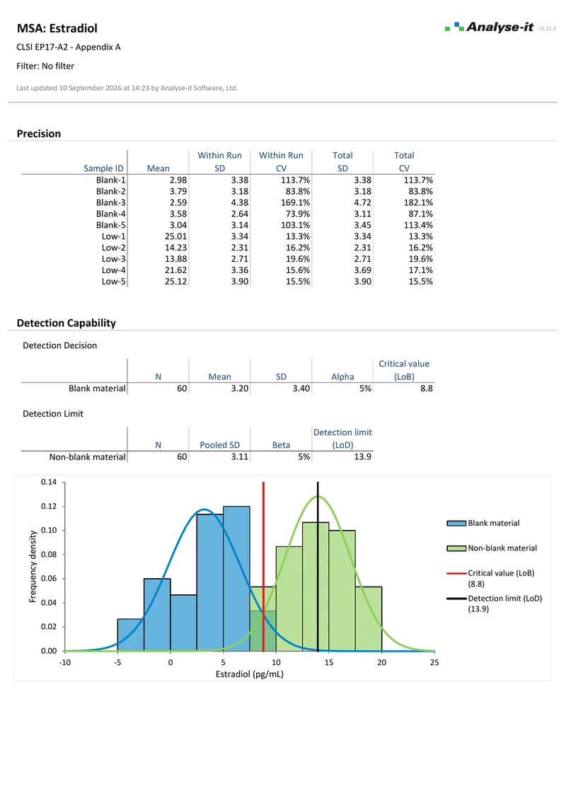 2 pages
EP17-A2 — Appendix A
2 pages
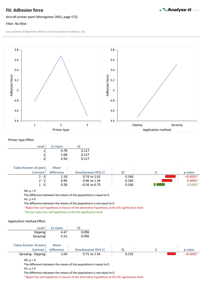
EP17-A2 — Appendix AChanging pH, then temperature, then flow rate, one at a time from a fixed baseline, cannot detect that a pH shift only matters when the column is warm. The interactions are usually the reason for a robustness study, and a one-factor-at-a-time table is structurally incapable of finding them.
A factorial design varies them together, and the analysis is an ordinary multi-factor model. Analyse-it fits that model with main effect and interaction plots, so an effect that only appears in combination is visible rather than inferred. Judge each effect against a limit set in advance and the study answers the question the specification is really asking. Robustness testing covers how to plan the design and read the interactions it finds.
ANOVA and multi-factor models →Validation establishes that the method worked once, under the conditions you wrote down. Accreditation bodies want evidence it still works. In practice that means charting check standards, reference materials or replicate controls over time and having a rule that says when to act.
Which control chart you need depends on whether results arrive singly or in batches and how small a shift you must catch. A slow drift in a reference standard is usually easier to see on a CUSUM or EWMA chart than on a Shewhart one. Reading out-of-control signals covers the rule sets and the cost of adding too many.
For the uncertainty statement, the top-down approach builds the estimate from the intermediate precision and bias the validation has already produced, rather than from a component-by-component budget.
Calibration curves, robustness by factorial design and the general toolkit — regression, multi-factor ANOVA, hypothesis tests — are the Standard edition, which every edition includes. The validation characteristics themselves are the Method Validation edition. That edition covers nested precision with variance components, linearity and range, detection and quantitation limits, recovery against a reference material, and comparison against a reference method.
Ongoing monitoring — control charts, detection rule sets and process capability — is the Quality Control & Improvement edition. Ultimate holds validation and monitoring in one licence. The comparison table lists every analysis against every edition, and volume pricing is available for teams.
Every calculation is performed by Analyse-it — no Excel formulas and no third-party functions. The calculations are validated against the NIST Statistical Reference Datasets, CLSI reference datasets and thousands of internal test cases. That validation is the basis of the evidence you show an assessor. Analyse-it runs entirely within Excel on your PC, so client and pre-submission data stays inside your own controls. The validation file is the workbook: data, analysis and conclusion together, openable years later by a reviewer with no licence. The workbook carries no formulas, so what you reported is what you find when you reopen the file. How Analyse-it is developed and validated →
Try it on your own data first. The 15-day trial is every feature from all five editions — install it and start straight away.
Method Validation edition: US$ 475 per year or US$ 1155 for a perpetual licence. Every purchase carries a 30-day money-back guarantee. Need a quote for purchasing? Choose the licence on the pricing page and click Get a quote.