
For most method comparisons the right regression is Deming or Passing–Bablok, not ordinary least squares. Ordinary least squares is the line every spreadsheet will draw for you without being asked, and in a method comparison it is usually the wrong one. Regression is the next step once you accept that the correlation coefficient cannot tell you whether two methods agree.
The reason ordinary least squares fails is a single assumption, and understanding it tells you almost everything you need to pick the right procedure.
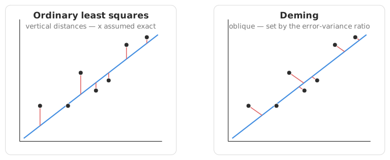
Ordinary least squares (OLS) fits a line by minimising the vertical distances from the points to the line. Minimising only the vertical distances is equivalent to assuming that the horizontal axis, your X method, is measured without error. Every bit of scatter is attributed to Y.
In a method comparison, that assumption is false. Both methods have measurement error; that is why you are comparing them. When error is present in X, OLS systematically underestimates the slope. The line is pulled flatter than the true relationship, an effect known as regression dilution or attenuation. You can end up reporting a proportional bias that is partly an artefact of your model rather than a property of your method.
There is one valid case for OLS: when X is a true reference method whose error is negligible relative to the range of values. Even then, Linnet (1993) showed that while the slope and intercept estimates carry little bias, their standard errors are underestimated. The confidence intervals are too narrow and the hypothesis tests too liberal. You get plausible-looking point estimates wrapped in confidence intervals you cannot trust. For most comparisons, use something other than OLS.
Deming regression is the errors-in-variables answer. Instead of minimising vertical distances, it minimises the distances to the line at an angle set by the ratio of the two methods’ error variances. Deming assumes both methods are measured with error, the realistic case, and returns a slope that is not attenuated.
What Deming requires in return is that variance ratio. If you measure your samples in replicate, Analyse-it estimates the error of each method from the data and computes the ratio for you. If you have only single measurements and no external estimate, a ratio of 1 is sometimes assumed as a default, which makes Deming equivalent to orthogonal regression.
The default is acceptable when the measuring range is wide relative to the measurement error. When the range is narrow it reintroduces bias and underestimated standard errors (Linnet 1998), so replicate measurement is worth the effort.
Weighted Deming (Linnet 1990) handles the common situation where precision is not constant across the interval. Typically the standard deviation grows with concentration, so the method has a roughly constant coefficient of variation (CV) rather than a constant SD. The model assumes each method’s SD is proportional to concentration, so the ratio of CVs is constant, and weights each point accordingly. If your scatter plot shows a band that fans out as values increase, this is the model you want.
Analyse-it computes confidence intervals for Deming parameters from a t-distribution, with standard errors from a jackknife procedure, which is reasonably robust in practice. Ordinary Deming also offers asymptotic standard errors.
Passing–Bablok takes a different route, estimating the slope as the shifted median of all possible pairwise slopes between points. The construction is non-parametric: it makes no assumption about the distribution of the measurement errors, and it is strikingly resistant to outliers. One or two aberrant points that would pull an OLS or Deming line away from the true relationship barely move a Passing–Bablok fit.
Passing–Bablok comes in two forms, and choosing the wrong one is a common error. Part I is for methods measured on the same scale, when the purpose is to test whether they are equal. Part III is for methods on different scales, or when the goal is to convert results from one method to the other rather than to test equality. Pick the one that matches your intent.
Passing–Bablok has trade-offs. Like the other procedures, it assumes the relationship is linear, so check that first. The procedure also implicitly assumes that the ratio of the two error variances equals the square of the slope. For similar methods, with a slope near 1, that means the two methods should have similar imprecision. Where one method is much noisier than the other, the slope estimate is biased. On very large datasets the all-pairwise-slopes computation is heavier, though on modern hardware this rarely matters.
| Ordinary least squares | Deming | Passing–Bablok | |
|---|---|---|---|
| Error in X | Assumed to be none | Allowed for, via the variance ratio | Allowed for, but assumes the variance ratio equals the slope squared |
| What it minimises | Vertical distances | Distances at an angle set by the variance ratio | Nothing — the slope is the shifted median of all pairwise slopes |
| Distribution assumed | Normal errors | Normal errors | None |
| Sensitive to outliers | Yes | Yes | No |
| Non-constant precision | Needs weighting | Use weighted Deming | Handled by Part III on a log scale |
| Extra input required | None | The ratio of the two error variances | None |
| Use it when | The X method really is a reference with negligible error | Both methods have error and you can estimate the ratio | Distribution is doubtful, or outliers are present |
The two errors-in-variables procedures usually agree closely on clean data. Where they differ is instructive. A large gap between the Deming and Passing–Bablok slopes generally has one of two causes. Either an outlier is pulling the Deming fit, or the variance ratio does not hold across the range.
The differences are easiest to see on a single dataset. The CLSI EP09-A3 worked example at the bottom of this page compares two measurement procedures across a set of patient samples spanning the measuring interval. The workbook fits five regressions to the same data: ordinary and weighted least squares, Deming and weighted Deming, and Passing–Bablok. Each reports the bias at a medical decision point with its confidence interval, and all but Passing–Bablok add a hypothesis test.
Laid side by side, the five fits show which distinction actually matters for this dataset:
Which distinction matters depends on the data and on the fit. Unweighted, this range is wide enough for ordinary least squares and Deming to agree. Weighted, the low end of the range dominates and the attenuation that Deming corrects reappears. Weighting moves the Deming slope only from 1.074 to 1.037, but the least-squares slope from 1.070 to 0.924. Fitting all five, rather than trusting one, is how you see which effect is actually in play.
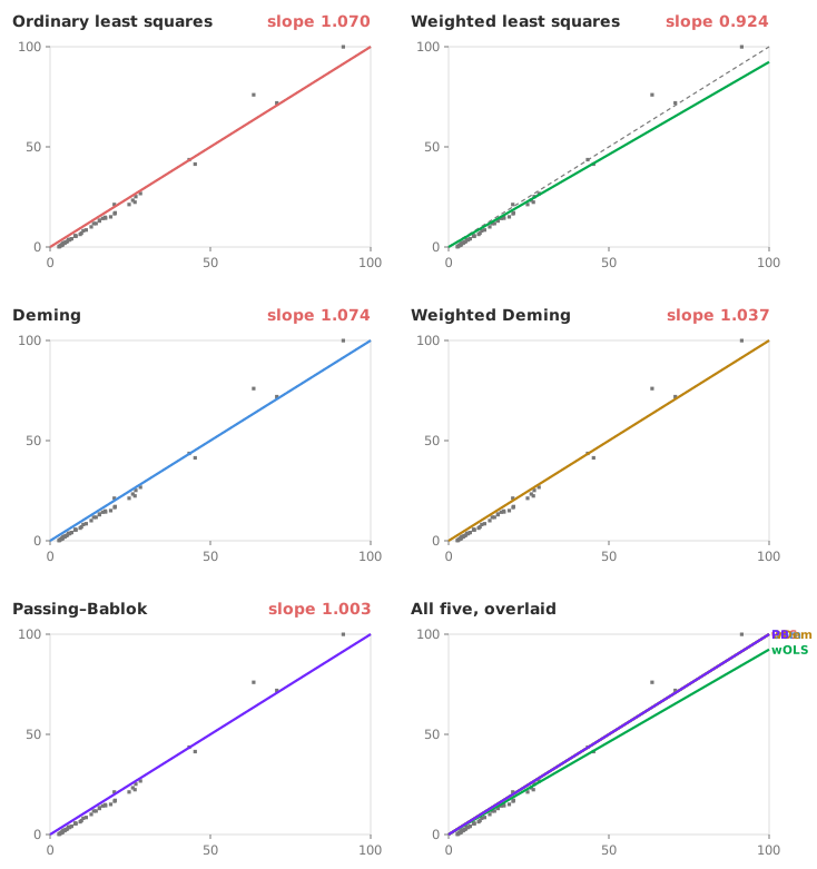
Open the workbook in the Analyse-it trial, run Method Comparison, and compare the fits. Each has its own scatter plot, parameter estimates and bias-at-decision-point estimate. Comparing them is the fastest way to build an intuition for when the choice matters and when it does not.
Work through it in this order. First, check linearity and residuals, before choosing any fit. Every procedure here assumes the relationship between the methods is linear. A CUSUM linearity test and a residual plot will tell you whether that holds. If the relationship bends, no choice of regression rescues it. You need to reduce or partition the measuring interval first.
Then choose:
| Situation | Procedure |
|---|---|
| X is a true reference method, error negligible | Ordinary least squares — cautiously, knowing the CIs run narrow |
| Both methods have error; errors roughly Gaussian; you want statistical efficiency | Deming |
| As above, but precision is proportional to concentration (constant CV, fanning scatter) | Weighted Deming |
| Outliers present, non-Gaussian errors, or you want the fewest assumptions | Passing–Bablok |
| Methods on different scales, or you are deriving a conversion | Passing–Bablok, Part III |
When two procedures are both appropriate, running them side by side is informative. Close agreement between, say, Deming and Passing–Bablok estimates is reassuring. A divergence is usually a signal worth investigating.
Download the CLSI EP09-A3 method comparison example workbook (.xlsx) — the same dataset fitted with ordinary and weighted least squares, Deming, weighted Deming, and Passing–Bablok, ready to open in the Analyse-it trial.
The example workbook is downloading.
It opens in Excel on its own — the data and the finished results are both in it. Analyse-it is what lets you change the analysis and re-run it, try the same study on your own data, or work through it to see how the software handles it.
Every feature from all five editions for 15 days.
Six recur often enough to be worth naming.
Using OLS out of habit. It is the spreadsheet default and the line most people were taught first, so it gets used without a second thought. In a method comparison its core assumption, an error-free X, is always violated. The default line is the wrong line for method comparison.
Defaulting the Deming variance ratio to 1 on a narrow range. Assuming equal error variances is fine when the measuring interval is wide relative to the measurement error. On a narrow range it reintroduces the very bias Deming exists to remove. Measure in replicate and let the ratio be estimated from the data.
Choosing the wrong Passing–Bablok variant. Part I tests equality on the same scale. Part III converts between scales. Reaching for Part I when you are really deriving a conversion, or vice versa, gives you a technically valid fit answering the wrong question.
Assuming the same choice applies to calibration. The weighting question is the same, but a calibration curve is fitted in one direction and used in the other. See fitting a calibration curve.
Skipping the linearity and residual checks. Every regression here assumes linearity. Fit without checking, and a curved relationship can look like a clean slope with a misleading bias estimate. Check linearity before you trust any parameter.
Reading a high correlation as justification for OLS. A near-perfect r says your sample range is wide relative to the measurement error. A high r does not make ordinary regression the right model, and the OLS confidence intervals still ignore the error in X. See why correlation is the wrong statistic.
Whichever fit you choose, the slope and intercept are intermediate results. The number a reviewer, an auditor or a clinician needs is the bias at the decision points that matter, with a confidence interval, tested against an allowable difference. The regression is how you estimate that bias without distortion. Matching the fit to the error structure of your data keeps the comparison sound; a line that ignores the error structure can look tidy and still mislead.
Analyse-it offers all five in its method comparison analysis, on your own data, inside Excel:
Every feature from all five editions for 15 days. Method comparison is in the Method Validation and Ultimate editions, from US$ 475 a year. The Medical edition covers Bland–Altman agreement, but not the regression fits or bias at decision points. Validated against NIST and CLSI reference datasets. Full detail in the method comparison reference guide.