
The correlation coefficient is the wrong statistic for a method comparison, yet it is still one of the most commonly reported. Open a validation report, a reagent evaluation or a manuscript comparing a new assay against a predicate, and somewhere near the top you will find r. The figure usually comes with a reassuring string of nines after the decimal point, offered as evidence that the two methods “agree well”.
A high correlation is evidence of no such thing. Bland and Altman made the point in 1986, and decades later the habit persists.
The correlation coefficient quantifies the strength of linear association between two variables: the tendency for one to increase as the other increases. Agreement is a different property entirely: whether the two methods give the same value for the same sample.
The two diverge immediately. Suppose a new method reads exactly double the reference method across the whole measuring interval. Every point falls precisely on a straight line. The correlation is a perfect 1.00. Yet the methods disagree by 100% at every concentration. A constant offset behaves the same way. If the new method reads 5 units high everywhere, r is still 1.00 while a clinically important bias goes entirely undetected. Correlation is blind to the systematic errors (proportional and constant bias) that a method comparison exists to detect.
The point is easiest to see in one picture. Take a dataset that spans a wide range, where the new method reads consistently high, and compute r. The correlation is near-perfect, while the difference plot of the same data shows the bias immediately. The same data lead to opposite conclusions, and only the difference plot is useful.
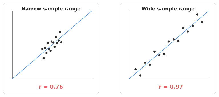
The correlation coefficient depends on the range of concentrations you sampled, which is the more subtle problem. Range dependence makes r look like a property of the two methods, when it is really a property of your sample.
The correlation coefficient is, in effect, the ratio of the variation between your samples to the total variation, measurement error included. Spread your samples across a wider concentration range and the between-sample variation grows while the measurement error stays put. r rises, even though nothing about the methods’ agreement has changed. Pick a narrow range and the same methods will produce a mediocre-looking r.
The practical consequence is that a high correlation can be manufactured by selecting samples across a broad interval. Two studies of the same two methods can report very different coefficients purely because of sample selection. A number that moves around based on how you chose your specimens is not telling you about the methods.
Reporting a p-value alongside r only compounds the problem. The null hypothesis being tested is that the true correlation is zero: that the two methods are unrelated. Two procedures measuring the same analyte are, of course, related. Rejecting that null tells you nothing you did not already know before collecting a single sample. A tiny p-value here is not a finding; it merely restates the obvious.
There is something to this one, provided you are precise about what it claims. The rule is sometimes attributed to Stöckl and Thienpont, and is referenced in older CLSI guidance. The heuristic holds that once r exceeds about 0.975, the range of true values is wide relative to measurement error. The slope from ordinary least squares regression is then not badly biased by error in the X variable.
Read carefully, that is a statement about range adequacy, not about agreement, and not a justification for using ordinary regression as your comparison. With a full complement of proper errors-in-variables procedures available, there is no reason to rely on a loose guideline about when an inappropriate model becomes tolerable. Use the coefficient, if at all, as a rough check that your samples span an adequate interval, never as your principal result.
The alternatives are more informative and easier to interpret, because they speak in the units your readers care about.
A difference plot, as described by Bland and Altman, plots the difference between the methods against the best estimate of the true value. The plot shows the bias directly, whether that bias is constant or grows with concentration, and it exposes outliers and non-constant scatter that a correlation coefficient hides completely. No other single picture in a method comparison is as useful.
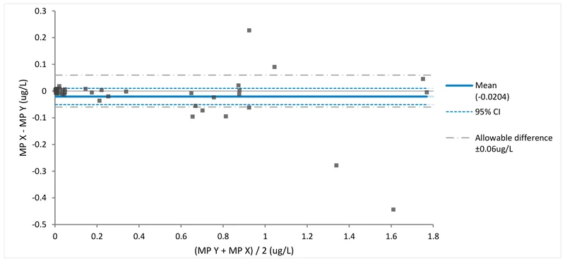
Limits of agreement turn that plot into an interval: the range within which most differences between the two methods are expected to fall. When one method is a reference, that interval is a usable estimate of total error.
An appropriate regression procedure estimates constant and proportional bias. From the fit you can predict the bias at the medical decision points that matter, with confidence intervals and equivalence tests against an allowable difference. Use Deming or Passing–Bablok rather than ordinary least squares, for reasons the regression guide covers.
None of these can be inflated by widening the sample range. None is blind to systematic error. Every one of them answers the real question: when these two methods measure the same sample, how far apart are the answers, and does that difference matter?
A correlation coefficient was never built to answer that question.
Analyse-it runs the analyses that answer the agreement question, on your own data, inside Excel:
Every feature from all five editions for 15 days. Method comparison is in the Method Validation and Ultimate editions, from US$ 475 a year. The Medical edition, from US$ 340 a year, covers Bland–Altman agreement, but not the regression fits or bias at decision points. Validated against NIST and CLSI reference datasets. Full detail in the method comparison reference guide.