
A calibration curve is the fitted relationship between a method’s response and known concentrations. You prepare standards, measure the response of each and fit a curve through the points. From then on the curve runs backwards: an unknown sample produces a response, and you invert the fit to get its concentration. That inversion is what makes calibration different from ordinary regression. The quantity you care about, the estimated concentration, is not the quantity the fit was optimised for.
Start with the simplest model the data support, and let the residuals decide whether it is enough. A straight line is right for many detectors over a limited range. A quadratic fits gentle curvature. Immunoassays and other binding assays are usually sigmoidal and need a four- or five-parameter logistic. Forcing a straight line through the linear-looking middle throws away both ends of the working range.
Do not add terms simply because the fit improves. Every extra parameter buys a closer pass through the calibrators you happen to have measured. A curve that follows its own calibration noise will estimate unknowns worse, not better. The model should reflect the response mechanism, not the scatter of one run.
A four- or five-parameter logistic is a different class of problem from everything else here. It is non-linear in its parameters, so fitting one takes iterative non-linear least squares rather than the algebra that fits a least-squares line. Iterative fitting of this kind is what dedicated immunoassay curve-fitting software is for; Analyse-it has no non-linear least-squares facility and does not fit 4PL or 5PL curves. The rest of this guide covers the models least squares can fit: the straight line, polynomials to 6th order and the linearisable forms — logarithmic, exponential and power. Between them, the straight line, the polynomials and the linearisable forms cover most chromatographic, spectrophotometric and electrochemical calibrations.
One naming collision causes confusion. A 4PL is not the four-parameter variance function used in a precision profile. A variance function models imprecision — SD or CV — against concentration, and is what sets the limit of quantitation. A 4PL models response against concentration. The two share a number and nothing else.
Weighting is the decision that matters most, and one that is often left at its default. Ordinary least squares minimises the sum of squared residuals in the response units. The fit treats an error of 100 units at the top of the curve as exactly as important as an error of 100 units at the bottom. Detector response is almost always heteroscedastic: absolute variability grows with concentration, so the top standards have far larger residuals in absolute terms. Under unweighted fitting those top standards dominate the fit.
The consequence is a curve pulled towards the high standards and fitted poorly at the low end. Yet the low end is where the limit of quantitation lives and where most clinically or environmentally interesting samples sit.
Weighting each point by 1/x² makes a 5% error count the same everywhere on the curve, which is right when the CV is constant. Weighting by 1/x suits variance that rises in proportion to concentration. Where replicate data are available to estimate it, the reciprocal of the variance is better still. The same logic drives the choice between ordinary and weighted regression in method comparison: constant SD means unweighted, constant CV means weighted.
The way to decide is to look. Run replicates at several levels, plot the standard deviation of the response against concentration, and see whether it is flat or rising. A rising profile means weighting.
In Analyse-it, Fit Model takes an optional weight variable, so a calibration can be fitted by weighted least squares with weights held in a worksheet column. The dilution-series linearity analysis can weight its fits by the variance at each level. Method comparison offers weighted least squares and weighted Deming regression.
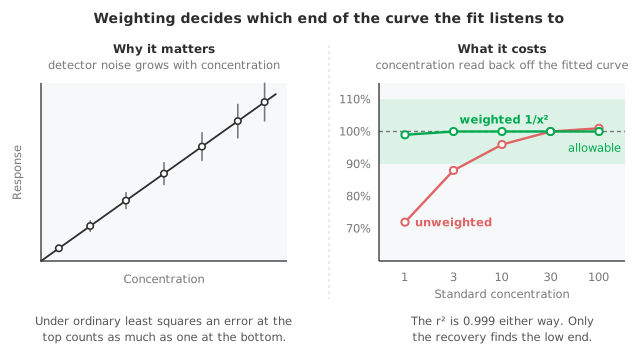
A calibration with an r² of 0.999 can still be systematically wrong at the concentrations you care about. The coefficient measures how much of the variation in response the model accounts for. Over a range spanning two or three orders of magnitude, r² will be close to one for almost any monotonic fit. Even a straight line through an obviously curved set of points will score close to one. The same failure makes correlation the wrong statistic for method comparison: a measure of association is not a measure of agreement.
What does the job is the residual plot. Plot residuals against concentration and look for structure. Random scatter around zero means the model is adequate. A curve, a fan or a run of points on one side means it is not, whatever r² says.
Where you have replicates at each level, a lack-of-fit test separates the two questions properly. The test compares the variation of points around the fitted curve with the variation between replicates at the same level. The result tells you whether the misfit is larger than measurement noise can explain.
Since the curve is used in inverse, test it in inverse. Take each calibrator, read its concentration back off the fitted curve, and compare that with its assigned value. This back-calculation gives a recovery at every level, and exposes exactly what the residual plot only hints at. A curve that is fine at the top and reads 20% low at the bottom standard shows that here, in units anyone can act on.
Set an acceptance criterion for that recovery before you look, level by level, and expect a wider tolerance at the lowest standard than in the middle. A calibrator that fails its own recovery check should not be dropped just to improve the fit. The reason it failed is useful data.
In Analyse-it, a calibration fitted as a straight line, a polynomial or a logarithmic, exponential or power curve can be used backwards directly. Fit Model predicts X given Y, reporting the concentration for a given response with a confidence interval. Put the recovery column beside the back-calculated concentrations. The same inverse prediction is reported for logistic and probit models, where the question is the concentration at a given probability. See probit analysis for the limit of detection.
The curve is only evidence over the interval the standards covered. Extrapolating above the top calibrator or below the bottom one estimates concentrations from a model shape that was never tested there. Nothing in the data limits how large the error can be.
The working range is bounded at the bottom by the higher of the limit of quantitation (the concentration where imprecision first meets your goal) and the lowest calibrator. At the top it is bounded by the highest calibrator. Results outside it are reported as below or above the range rather than as numbers. The measuring interval and the reportable range covers where dilution extends the range and where it does not.
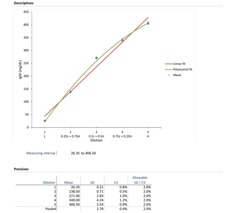
Download the dilution-series linearity example workbook (.xlsx) — five levels with replicates, fitted with linear and polynomial models, with the deviation from linearity assessed at each level. The workbook is framed as a CLSI EP06 linearity study rather than a calibration, but the structure is the same. Both have known levels, replicates, a fitted model and a fit judged level by level.
The example workbook is downloading.
It opens in Excel on its own — the data and the finished results are both in it. Analyse-it is what lets you change the analysis and re-run it, try the same study on your own data, or work through it to see how the software handles it.
Every feature from all five editions for 15 days.
Leaving the weighting at unweighted. An unweighted fit is decided by the top standards and reads badly at the bottom when response variability grows with concentration. The bottom of the range is usually where the samples that matter are.
Judging the fit by r². It will be high for a curved set of points fitted with a line. Read the residual plot, and test lack of fit against replicate variation where you can.
Adding terms to improve the fit. A higher-order polynomial passes closer to the calibrators and estimates unknowns worse. Match the model to the response mechanism.
Extrapolating beyond the standards. The curve is evidence only between the lowest and highest calibrator. Outside that, report the result as beyond the range.
Dropping an inconvenient calibrator. Removing a level because it spoils the fit hides the problem rather than solving it. Investigate why it failed.
Analyse-it fits the model and reports what shows whether it holds, inside Excel:
Every feature from all five editions for 15 days. Model fitting is in every edition, from US$ 155 a year; the dilution-series linearity analysis, which weights each level by its variance and tests the deviation level by level, is in the Method Validation and Ultimate editions, from US$ 475 a year. Validated against NIST and CLSI reference datasets. See assessing linearity of a measurement procedure for judging deviation against an allowable limit, or the trueness and linearity reference guide for the technical detail.