
The classical limit of detection is the limit of blank plus a multiple of the low-level SD. The calculation assumes the method returns a continuous signal you can take a standard deviation of. Many assays do not. A qualitative molecular test returns detected or not-detected. A nucleic-acid assay either amplifies or it does not. For these, detection is a probability that rises with concentration. The detection limit is the concentration at which that probability reaches an agreed level, conventionally 95%. Probit analysis is how you estimate it.
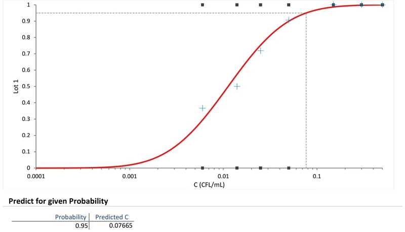
Test replicates of a dilution series. At each concentration, record the proportion that come back positive. Far below the detection limit almost nothing amplifies, and far above it almost everything does. In between, the hit rate climbs from near 0 to near 1, and plotted against concentration it traces an S-shaped dose-response curve. The detection limit is a specific point on it: the concentration where the hit rate crosses 95%.
Probit regression fits that S-curve. The model links the probability of detection to concentration, usually log concentration, through the inverse of the cumulative standard normal distribution, which is the probit link. The fit turns the scattered hit rates at each level into a smooth curve. From the fitted model you predict the concentration corresponding to any chosen detection probability, and report its confidence interval. The fit uses every replicate at every level. The detection limit it gives is therefore far more stable than reading off by eye the level where hits happen to cross 95%.
Detection can differ between reagent lots or instruments. The model is typically fitted per lot, and the detection limits compared. The worked example below does exactly this across three reagent lots, fitting a probit curve to each and predicting the concentration at 95% detection for every one.
| Your data are… | Use… |
|---|---|
| Continuous signals from blank and low-level samples | Parametric (or precision-profile) LoD |
| Detected / not-detected outcomes across a dilution series | Probit regression |
The two are not competing estimates of the same thing; each suits a different kind of data. If your assay produces a number, take the standard-deviation route. If it produces a yes/no across dilutions, the hit rate is your data and probit is the tool.
Download the CLSI EP17-A2 probit example workbook (.xlsx) — probit regression fitted to a dilution series across three reagent lots, with the concentration giving 95% detection for each, ready to open in the Analyse-it trial.
The example workbook is downloading.
It opens in Excel on its own — the data and the finished results are both in it. Analyse-it is what lets you change the analysis and re-run it, try the same study on your own data, or work through it to see how the software handles it.
Every feature from all five editions for 15 days.
Reading the detection limit off the raw hit rates. The level where replicates happen to cross 95% is noisy. Fit the probit model and predict from the curve, with a confidence interval.
Too few levels around the transition. The curve is defined by the region where the hit rate climbs. Place most dilutions there, not where detection is already certain or impossible.
Pooling across lots that differ. Detection can vary by reagent lot or instrument. Fit each separately and compare, rather than averaging a difference away.
Applying probit to continuous data. If the assay returns a signal, use the parametric or precision-profile method. Probit is for detected/not-detected outcomes.
Analyse-it fits probit regression for detection capability, inside Excel:
Every feature from all five editions for 15 days. Probit regression is part of Fit Model in the Standard edition, so it is in every Analyse-it edition, from US$ 155 a year. The other detection capability methods are in the Method Validation and Ultimate editions, from US$ 475 a year. Validated against NIST and CLSI reference datasets. See the LoB, LoD and LoQ guide, or the detection capability reference guide.