
Robustness testing varies the method’s parameters on purpose and checks that the result does not move more than you can tolerate. The changes are small, representing the drift that will happen anyway in routine use. Temperature, pH, flow rate, wavelength, incubation time, reagent lot, column batch: whichever of these the method is plausibly sensitive to. Analyst and day effects belong to intermediate precision instead; see the precision components.
ICH Q2(R2) and Q14 expect robustness to be evaluated, usually during development and before the validation study. Robustness is also where system suitability criteria come from. A parameter the method turns out to be sensitive to is one you have to control tightly and say so in the procedure. A parameter it tolerates is one you can stop worrying about.
The intuitive approach is to hold everything fixed, move one parameter, see what happens, put it back, and move the next. One factor at a time is inefficient, and worse, it cannot detect an interaction.
An interaction is where the effect of one factor depends on the level of another. Suppose the method tolerates a slightly high temperature and a slightly low pH, but recovery collapses at high temperature and low pH together. Varied one at a time, each change looks harmless, and the combination that breaks the method is never tested. Routine use varies several parameters at once, so that combination will eventually occur.
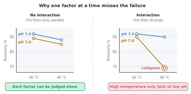
A factorial design tests every combination of the factor levels. With three factors at two levels each (low and high, either side of nominal), that is eight runs. Those eight runs estimate all three main effects and every interaction between them. To test the effects you also need an estimate of error: replicate the design, add centre points or treat the three-way interaction as error. Compared with one-factor-at-a-time, the factorial design gives more information from a similar number of runs. Every run contributes to the estimate of every effect rather than to just one.
Where there are many candidate parameters, a screening design tests a fraction of the combinations to identify which few factors matter. The cost is aliasing. In the smallest designs, such as Plackett–Burman, a main effect cannot be separated from two-factor interactions. Use at least a resolution IV design if two-factor interactions are a concern, and follow up any factor that shows an effect. The trade is usually right, because robustness is a screening question. The goal is to find the parameters that need controlling, not to characterise the response surface in detail.
Choose the levels to represent realistic deviation, not extremes. If the procedure says 37 °C and the incubator holds ±1 °C, test 36 and 38. Testing 30 and 45 will almost certainly find an effect, and will tell you nothing about whether the method is robust in service.
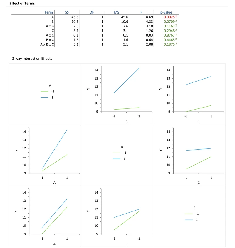
Fit a model with each factor as a term and the crossed terms for their interactions. The model gives the effect of each factor on the result, the effect of each combination and a test of each against the residual variation. A main effects plot shows the size and direction of each factor’s influence. An interaction plot shows where the effect of one factor depends on the other. Non-parallel lines are the signature.
Read the effect sizes before the p-values. With enough replication a trivial effect becomes statistically significant. A significant effect that shifts the result by a tenth of your allowable variation is not a robustness problem. The question is not whether a factor has any effect, since everything has some effect. The question is whether that effect, over the realistic range, is large enough to matter. Judge it against a limit you set beforehand, from an allowable total error figure or an equivalent specification.
Conversely, a large effect that misses significance because the study was small is not evidence of robustness. Report the effect with its confidence interval and judge that interval against your limit, rather than treating a p-value as the answer.
A factor with an effect too large to tolerate does not mean the method has failed. Such a factor marks a parameter that needs a tighter specification, and the robustness study has just told you how tight. Narrow the permitted range until the effect across it falls inside your limit. Then write that range into the procedure and, where it can be monitored, into the system suitability criteria.
The factors that turn out not to matter are equally useful. Their results justify the tolerances in the written method, and show that a small deviation in routine use needs no investigation.
Download the three-factor example workbook (.xlsx) — Montgomery’s surface-finish 2³ factorial, ready to open in the Analyse-it trial. Every two- and three-way interaction is fitted, with main effect plots and two- and three-way interaction plots. A robustness screen produces the same analysis. A two-factor example shows the analysis with a single crossed term.
The example workbook is downloading.
It opens in Excel on its own — the data and the finished results are both in it. Analyse-it is what lets you change the analysis and re-run it, try the same study on your own data, or work through it to see how the software handles it.
Every feature from all five editions for 15 days.
Varying one factor at a time. It cannot detect interactions, and interactions are the failures that surprise people. Vary the factors together.
Choosing unrealistic levels. Extreme settings guarantee an effect and answer nothing. Use the deviation the method will actually meet.
Reading p-values instead of effect sizes. Statistical significance and practical importance are different questions. Judge the size of the effect against a pre-set limit.
Leaving interactions out of the model. Fitting main effects only pushes any interaction into the residual, which inflates the error term and hides the effect you were looking for.
Stopping at the finding. A sensitive parameter should end up with a tighter range in the written procedure, not just a note in the validation report.
Analyse-it fits the factorial model on your own runs, inside Excel:
Every feature from all five editions for 15 days. Model fitting is in every edition, from US$ 155 a year. Validated against NIST and CLSI reference datasets. See precision components explained for separating sources of variation in a nested rather than crossed design.