
A cut-off, or decision threshold, is the value that divides the results of a quantitative test into positive and negative. The area under the ROC curve summarises a test’s discrimination without one, but the moment the test enters routine use, someone has to draw that line.
For most markers a higher value is the more suspicious one, so results above the line are positive and those below it negative. For some the association runs the other way, and it is a low value that signals disease, which simply mirrors the rule.
Where that line goes is not a statistical detail. The cut-off fixes the balance of missed cases against false alarms. Different clinical situations want that balance struck in very different places.
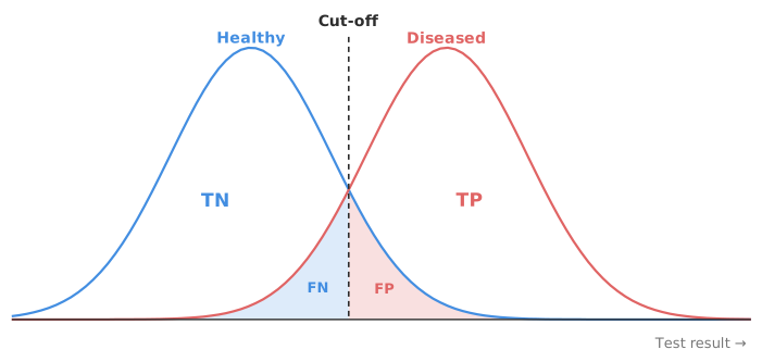
The most common rule is Youden’s index: choose the cut-off that maximises sensitivity plus specificity minus one. Geometrically it is the point on the ROC curve furthest above the diagonal, where sensitivity and specificity together are highest. Simple and needing nothing but the ROC data, Youden’s index is a reasonable default when you have no strong reason to prefer catching cases over avoiding false alarms.
Even-handedness is Youden’s assumption. The index weights sensitivity and specificity equally. Equal weighting minimises the cost of errors only when a missed case and a false alarm cost the same and the prevalence is 50%. In medicine the two costs are rarely equal. Missing an aggressive, treatable cancer is not interchangeable with an unnecessary follow-up scan. A rule that treats them as such will put the cut-off in the wrong place for the clinical reality.
When the two errors carry different costs, the optimal cut-off shifts. The direction is intuitive. If a missed case is far worse than a false alarm, you move the cut-off to catch more cases, accepting more false positives. Prevalence works the same way. When disease is rare, the same relative cost produces many more false positives per true case, which moves the optimal cut-off towards higher specificity.
The formal version chooses the cut-off where the ROC curve’s slope equals a value set by the costs and the prevalence:
slope = (CFP / CFN) × (1 − p) / p
Here CFP and CFN are the costs of a false positive and a false negative, each measured against the correct call, and p is the prevalence. With equal costs and a prevalence of 10%, the optimal slope is 9, far steeper than the slope of 1 at Youden’s cut-off. The practical version is simply to state your relative cost of the two errors and let it move the line. Equal weighting should be something you chose, not a default.
Often the cleaner approach is to fix the operating characteristic the clinical role demands, and read off the other. For a screening test that must not miss cases, you set a required sensitivity, say 95% or 99%, and report the specificity at that point. For a confirmatory test that must not falsely label healthy people, you set a required specificity instead. Fixing the requirement in advance makes the clinical priority explicit and the trade-off visible, rather than hiding both inside a single “optimal” number.
One common mistake inflates the reported performance of a cut-off chosen from the data. Choose the threshold that maximises performance on your data, then report the sensitivity and specificity at that threshold from the same data, and both figures are biased upward. The cut-off is fitted partly to the noise in that sample, so the reported figures overstate how the test will perform. On a fresh sample the same cut-off will usually look worse.
The correction is to separate choosing the cut-off from estimating its performance. Select on one dataset and evaluate on another, or use cross-validation or bootstrapping to estimate the optimism and discount for it. At the very least, report the sensitivity and specificity at your chosen cut-off with their confidence intervals. With the small diseased groups typical of these studies the intervals are often wide. Even so, the intervals understate the uncertainty, because they do not allow for choosing the cut-off on the same data.
The workbook below plots sensitivity and specificity against every cut-off for an oxidised-LDL marker, beside its ROC curve. Read the decision threshold plot to see the two rates trade against each other as the cut-off moves. In the trial, ask for an optimal cut-off with your own costs and prevalence, and recalculate to see where it falls.
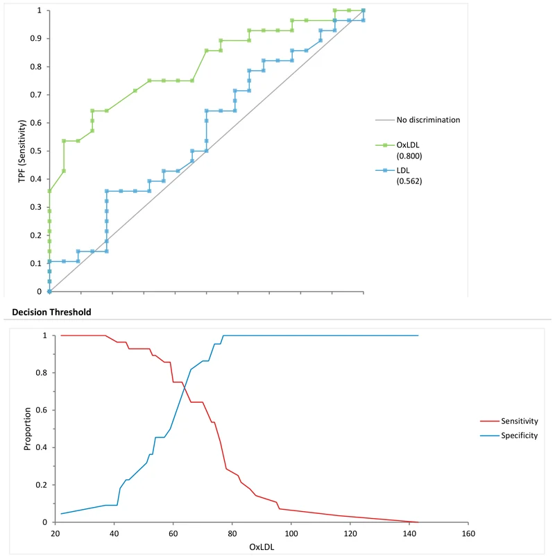
Download the CLSI EP24-A2 diagnostic performance example workbook (.xlsx) — ROC curves for OxLDL and LDL with a decision threshold plot of sensitivity and specificity across every OxLDL cut-off, ready to open in the Analyse-it trial.
The example workbook is downloading.
It opens in Excel on its own — the data and the finished results are both in it. Analyse-it is what lets you change the analysis and re-run it, try the same study on your own data, or work through it to see how the software handles it.
Every feature from all five editions for 15 days.
Defaulting to Youden without thinking about costs. Youden is right only when the two errors cost the same and the prevalence is near 50%. Decide whether that holds before you accept its cut-off.
Reporting performance at a cut-off chosen on the same data. The optimism is built in. Validate the cut-off on independent data, or estimate and discount the optimism.
Quoting performance at a cut-off without confidence intervals. The sensitivity and specificity at the operating point are estimates. With a small diseased group they can be very uncertain. Report the intervals.
Using one cut-off for two purposes. A screening threshold and a confirmatory threshold answer different questions. One number rarely serves both.
Analyse-it selects and reports the cut-off from your own data, inside Excel:
Every feature from all five editions for 15 days. Diagnostic performance is in the Medical, Method Validation and Ultimate editions, from US$ 340 a year. Validated against NIST and CLSI reference datasets. Start with the ROC and AUC guide, or the diagnostic performance reference guide for the technical detail.