
Capability indices translate a process spread into an expected fraction outside the specification, and the translation runs through the normal distribution. The calculation assumes the tails of the process fall away at the rate a bell curve predicts. When the real distribution is skewed or bounded, its tails behave differently, and an index that assumes normal tails no longer means what it appears to mean.
Many real characteristics are not symmetric. Anything physically bounded at zero piles up against the bound and trails off to one side. Typical examples are flatness, an impurity concentration, a time to event and a particle count. The skew is strongest when the process runs close to the bound. Fit a symmetric normal curve to that shape and one tail is forced to describe data that are not there. The other tail understates the data that are.
Cpk is read as a statement about the tail beyond the nearer limit, so a mismatched tail is exactly the error that matters. A skewed process can look comfortably capable while still producing defects on its long side, or look marginal when it is fine.
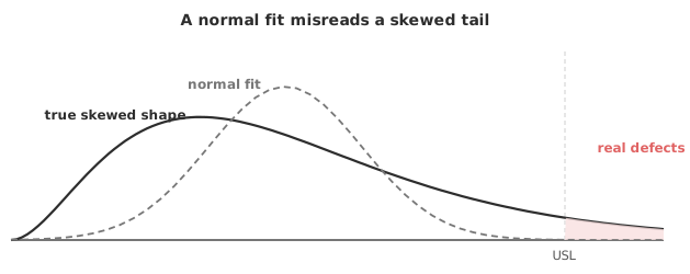
The first step is to look. A histogram with a normal overlay and a normal Q-Q plot will usually show skew at a glance. A formal normality test (Shapiro–Wilk or Anderson–Darling) puts a number on it. A clear departure from normality is the signal to stop reading the ordinary capability index at face value and to model the distribution properly. Do not skip this because the index “looks fine”. A healthy Cpk computed on skewed data is precisely the trap.
The practical route is to transform the data onto a scale where they are approximately normal. A Box–Cox or other power transformation finds the exponent that best straightens the distribution. Then compute capability on that scale, carrying the specification limits through the same transformation so that the index and the limits stay together.
The field recognises a second approach as well: fitting a non-normal distribution to the shape of the data and reading the out-of-specification fraction from it directly. Either route gives a defect estimate from a model that matches the tail you actually care about, rather than one imposed on it.
A capability index on transformed data is only interpretable with the transformation stated. Record the transformation used (the exponent, say) alongside the index. A reviewer needs to know that the 1.4 you are quoting came from a log scale, not the raw one. The reviewer also needs to know that the specification limits were transformed to match.
Download the process capability example (.xlsx) — includes a histogram, a normal Q-Q plot and a Shapiro–Wilk normality test to judge the distribution before reading the index, ready to open in the Analyse-it trial.
The example workbook is downloading.
It opens in Excel on its own — the data and the finished results are both in it. Analyse-it is what lets you change the analysis and re-run it, try the same study on your own data, or work through it to see how the software handles it.
Every feature from all five editions for 15 days.
Assuming normality without checking. The index computes happily on any data; whether it means anything depends on the distribution. Test first.
Transforming the data but not the limits. Specification limits must go through the same transformation as the data, or the index compares two different scales.
Forcing normality on a bounded characteristic. A hard bound close to the process mean guarantees skew. Model it rather than pretend it away.
Quoting a transformed index without saying so. An index means different things on different scales. State the transformation used.
Analyse-it checks the distribution before it computes anything, inside Excel:
Every feature from all five editions for 15 days. Capability analysis is in the Quality Control & Improvement and Ultimate editions, from US$ 290 a year. Validated against published reference datasets and thousands of internal test cases. See Cp, Cpk, Pp and Ppk explained for the indices themselves.