Sigma level, Z-benchmark and PPM Capability indices, sigma levels and parts-per-million defect rates are three views of the same thing: how far the nearer specification limit sits from the process, measured in standard deviations. Convert between them and the numbers stop being jargon.

One quantity sits behind capability indices, sigma levels and defect rates: the number of standard deviations between the process mean and a specification limit. Read that distance off the normal curve and you get the expected fraction beyond the limit. Scale that fraction by a million and you get parts per million. Divide the distance by three and you get a capability index. Capability index, sigma level and PPM are one measurement in three forms.

Z-benchmark and the defect rate

Start with the distance from the process mean to the upper or lower specification limit (USL or LSL), in standard deviations. For the upper limit, Z_upper = (USL − mean) / σ, and for the lower, Z_lower = (mean − LSL) / σ. Feed either into the normal distribution and you get the expected proportion of output beyond that limit. Multiply by 1,000,000 and it becomes expected defects in parts per million (PPM).

A capability index is this distance divided by three, so the two are linked. A Cpk of 1.33 corresponds to a Z of about 4 on the nearer limit.

The Z-benchmark combines both limits into a single figure. Add the tails beyond each limit to get the total nonconforming fraction. The Z-benchmark is the one Z that would produce that same total from a single tail, so the benchmark is never larger than the nearer-limit Z. For a two-sided specification, quote the benchmark, not a single-limit figure. When one tail dominates, the benchmark and the nearer-limit Z are almost identical. When both tails contribute, the benchmark sits below the nearer-limit distance.

Sigma level, and the 1.5-sigma shift

The sigma level of Six Sigma is the same Z with one convention layered on. The convention assumes that a process mean drifts over the long term. The level is quoted as the short-term distance, and an allowance of 1.5 standard deviations is subtracted before the long-term defect rate is read.

A process whose short-term Z is 6 is quoted as a “six sigma” process, and its long-term defect rate is read at Z = 4.5. The shift is why the familiar figure for six sigma is 3.4 PPM. A literal six-standard-deviation tail would give a vanishingly small rate, about 0.001 PPM. The 1.5-sigma allowance is a modelling assumption about long-term drift, not a law. If your own data give you the long-term spread directly, you do not need it.

Short-term and long-term must match the question

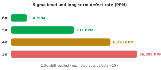
State whether you use the short-term or long-term spread. The choice decides which number you get. The short-term Z, from within-subgroup variation, describes the process at its best and pairs with Cp/Cpk. The long-term Z, from the overall spread, describes what actually shipped and pairs with Pp/Ppk. Quoting a short-term sigma level against a long-term defect rate mixes two questions. The figure answers neither.

Downloads

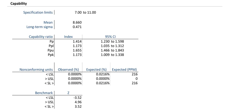
Download the process capability example (.xlsx) — copper plating with Z-benchmarks and observed and expected nonconforming units. The expected rate is 216 PPM, all below the lower limit. The workbook is ready to open in the Analyse-it trial.

Common mistakes

Quoting a sigma level without the shift convention. A “six sigma” process means 3.4 PPM because of the 1.5-sigma allowance. State whether the shift is applied, or the number is ambiguous.

Mixing short-term and long-term. Capability uses within-subgroup spread; performance uses overall spread. Keep the sigma level and the PPM on the same footing.

Quoting one tail for a two-sided specification. The total defect rate sums the tails beyond both limits. Report the Z-benchmark, which already combines them, not a single-limit figure.

Reading PPM from a non-normal process. The Z-to-PPM conversion runs through the normal curve. On skewed data, model the distribution first or the PPM is fiction.

Treating 3.4 PPM as a measured rate. It is what a 4.5-sigma tail predicts under an assumption about drift, not a count of observed defects. Report the observed rate too.