
1. Statistical Reference Guide
  2. Control charts
  3. Time-weighted control charts

CUSUM & EWMA Control Charts in ExcelA time-weighted control chart detects small shifts in a process mean.

Time-weighted control charts combine information from the current and past observations. They are more sensitive to detecting small shifts in the process mean than a Shewhart chart, but slower at detecting large shifts.

The charts only monitor the process mean; monitoring the process variability requires the use of some other technique.

Uniformly Weighted Moving Average (UWMA) chart

A uniformly weighted moving average (UWMA) chart is a type of control chart used to monitor small shifts in the process mean. It uses the average of a number of consecutive observations.

The UWMA chart plots the moving average for individual measurements or subgroup means.


UWMA shewhart chart

Given a series of observations and a fixed subset size, the first element of the moving average is the average of the initial subset of the number series. Then the subset is modified by "shifting forward"; that is, excluding the first number of the series and including the next number following the subset in the series. The next element of the moving average is the average of this subset. This process is repeated over the entire series creating the moving average statistic.

The UWMA requires:
  • A fixed subset size, the number of successive observations (span) in the moving average. Span must satisfy 1 < span ≤ n. Default span=3.

    A small span reduces the influence of older observations; a large span slows the response to large shifts. In general, the magnitude of the shift to detect and the span are inversely related.

Each point on the chart represents the value of a moving average.

The center line is the process mean. If unspecified, the process mean is the weighted mean of the subgroup means or the mean of the individual observations.

The control limits are a multiple (L) of sigma above and below the center line. Default L=3. If unspecified, the process sigma is the pooled standard deviation of the subgroups, or the standard deviation of the individual observations, unless the chart is combined with an R-, S-, or MR- chart where it is estimated as described for the respective chart.

UWMA is sensitive to small shifts in the process mean, but is not as effective as either the CUSUM or EWMA (Montgomery 2012).

Exponentially Weighted Moving Average (EWMA) chart

An exponentially weighted moving average (EWMA) chart is a type of control chart used to monitor small shifts in the process mean. It weights observations in geometrically decreasing order so that the most recent observations contribute highly while the oldest observations contribute very little.

The EWMA chart plots the exponentially weighted moving average of individual measurements or subgroup means.

EWMA shewhart chart

Given a series of observations and a fixed weight, the first element of the exponentially weighted moving average is computed by taking the (1-weight) * previous EWMA + (weight * current observation). Then the current observation is modified by "shifting forward"; and repeating the calculation. This process is repeated over the entire series creating the exponentially weighted moving average statistic.

The EWMA requires:
  • A weight for the most recent observation. Weight must satisfy 0 < weight ≤ 1. Default weight=0.2.

    The "best" value is a matter of personal preference and experience. A small weight reduces the influence of the most recent sample; a large value increases the influence of the most recent sample. A value of 1 reduces the chart to a Shewhart Xbar chart. Recommendations suggest a weight between 0.05 and 0.25 (Montgomery 2012).

When designing an EWMA chart it is necessary to consider the average run length and shift to be detected. Extensive guidance is available on suitable parameters (Montgomery 2012).

It is possible to modify the EWMA, so it responds more quickly to detect a process that is out-of-control at start-up. This modification is done using a further exponentially decreasing adjustment to narrow the limits of the first few observations (Montgomery 2012).

Each point on the chart represents the value of the exponentially weighted moving average.

The center line is the process mean. If unspecified, the process mean is the weighted mean of the subgroup means or the mean of the individual observations.

The control limits are a multiple (L) of sigma above and below the center line. Default L=3. If unspecified, the process sigma is the pooled standard deviation of the subgroups, or the standard deviation of the individual observations, unless the chart is combined with an R-, S-, or MR- chart where it is estimated as described for the respective chart.

Because the EWMA is a weighted average of all past and the current observations, it is very insensitive to the assumption of normality. It is, therefore, an ideal replacement for a Shewhart I-chart when normality cannot be assumed.

Like the CUSUM, EWMA is sensitive to small shifts in the process mean but does not match the ability of a Shewhart chart to detect larger shifts. For this reason, it is sometimes used together with a Shewhart chart (Montgomery 2012).

Creating a UWMA control chart

Plot a UWMA control chart to determine if a process is in a state of statistical control.

  1. Select a cell in the dataset.
  2. On the Analyse-it ribbon tab, in the Statistical Analyses group, click Process Control, and then click UWMA
    The analysis task pane opens.
  3. In the Model drop-down menu:
    • If the data are individual observations, select Process variable .
    • If the data are rational subgroups, select Process variable with Subgroups.
  4. In the Process drop-down list, select the quality characteristic variable.
  5. If the data are collected in subgroups, in the Sample size group:
    • If the subgroups are identified by a variable, select Subgroup by identifier variable, and in the Id drop-down list, select the subgroup identifier variable.
    • If the subgroups are a constant size and formed by consecutive number of observations of the process variable, Subgroup size constant, and in the edit box, enter the number of consecutive observations per subgroup.
  6. Optional: If the data are individual observations, in the Id drop-down list, select an identifier variable
  7. In the Span edit box, type the number of consecutive values to compute the UWMA statistic.
  8. In the L edit box, type the multiple of the process sigma to define the control limits.
  9. Optional: To reset the value of the UWMA statistic after each out-of-control signal, select the Reset after out-of-control signal check box.
  10. Optional: To specify known process parameters, select the Known process parameters check box, and then in either or both the Mean and Standard deviation edit boxes, type the known value of the parameter.
  11. Optional: To show the process mean and sigma statistics, select the Show process statistics check box.
  12. Optional: To show the center and control limit statistics, select the Show process control statistics check box.
  13. Click Calculate.

Creating an EWMA control chart

Plot an EWMA control chart to determine if a process is in a state of statistical control.

  1. Select a cell in the dataset.
  2. On the Analyse-it ribbon tab, in the Statistical Analyses group, click Process Control, and then click EWMA
    The analysis task pane opens.
  3. In the Model drop-down menu:
    • If the data are individual observations, select Process variable .
    • If the data are rational subgroups, select Process variable with Subgroups.
  4. In the Process drop-down list, select the quality characteristic variable.
  5. If the data are collected in subgroups, in the Sample size group:
    • If the subgroups are identified by a variable, select Subgroup by identifier variable, and in the Id drop-down list, select the subgroup identifier variable.
    • If the subgroups are a constant size and formed by consecutive number of observations of the process variable, Subgroup size constant, and in the edit box, enter the number of consecutive observations per subgroup.
  6. Optional: If the data are individual observations, in the Id drop-down list, select an identifier variable
  7. In the Weight edit box, type the weight to be assigned to the current sample in the EWMA statistic.
  8. In the L edit box, type the multiple of the process sigma to define the control limits.
  9. Optional: To detect existing out-of-control situations quickly, select the Headstart check box, and in the a and f edit boxes, type the parameters.

    A value of a=0.3 and f=0.5 mimics a 50% headstart.

  10. Optional: To reset the value of the EWMA statistic after each out-of-control signal, select the Reset after out-of-control signal check box.
  11. Optional: To specify known process parameters, select the Known process parameters check box, and then in either or both the Mean and Standard deviation edit boxes, type the known value of the parameter.
  12. Optional: To show the process mean and sigma statistics, select the Show process statistics check box.
  13. Optional: To show the center and control limit statistics, select the Show process control statistics check box.
  14. Click Calculate.

CUmulative SUM (CUSUM) chart

A cumulative sum (CUSUM) chart is a type of control chart used to monitor small shifts in the process mean. It uses the cumulative sum of deviations from a target.

The CUSUM chart plots the cumulative sum of deviations from the target for individual measurements or subgroup means.
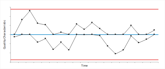

cusum plot

The CUSUM requires two parameters:
  • A reference value (k) specified in sigma units. k is often set to half the shift to be detected, in sigma units. Default k=0.5 which is equal to detecting a shift of 1 sigma.
  • The decision limit (h) specified in sigma units. Default h=5.
When designing a CUSUM chart it is necessary to consider the average run length and shift to be detected. Extensive guidance is available on suitable parameters (NIST 2012, Montgomery 2012).

It is possible to modify the CUSUM, so it responds more quickly to detect a process that is out-of-control at start-up. This modification is done using an initial CUSUM equal to half of the h parameter.

Like the EWMA, CUSUM is sensitive to small shifts in the process mean but does not match the ability of a Shewhart chart to detect larger shifts. For this reason, it is sometimes used together with a Shewhart chart (Montgomery 2012).

Creating a CUSUM control chart

Plot a CUSUM control chart to determine if a process is in a state of statistical control.

  1. Select a cell in the dataset.
  2. On the Analyse-it ribbon tab, in the Statistical Analyses group, click Process Control, and then click CUSUM
    The analysis task pane opens.
  3. In the Model drop-down menu:
    • If the data are individual observations, select Process variable .
    • If the data are rational subgroups, select Process variable with Subgroups.
  4. In the Process drop-down list, select the quality characteristic variable.
  5. If the data are collected in subgroups, in the Sample size group:
    • If the subgroups are identified by a variable, select Subgroup by identifier variable, and in the Id drop-down list, select the subgroup identifier variable.
    • If the subgroups are a constant size and formed by consecutive number of observations of the process variable, Subgroup size constant, and in the edit box, enter the number of consecutive observations per subgroup.
  6. Optional: If the data are individual observations, in the Id drop-down list, select an identifier variable
  7. In the k and h edit boxes, type the design parameters for the CUSUM chart.
    Note: k and h are specified in multiples of sigma and not in the data measurement units.
  8. Optional: To detect existing out-of-control situations quickly, select the Headstart check box, and in the Headstart h edit box, type the headstart value.

    Typically the headstart h is set to half the h value.

  9. Optional: To standardize the CUSUM statistic, so the control limits are constant regardless of the size of each subgroup, select Standardized plot.
  10. Optional: To reset the value of the CUSUM statistic after each out-of-control signal, select the Reset after out-of-control signal check box.
  11. Optional: To specify known process parameters, select the Known process parameters check box, and then in either or both the Mean and Standard deviation edit boxes, type the known value of the parameter.
  12. Optional: To show the process mean and sigma statistics, select the Show process statistics check box.
  13. Optional: To show the center and control limit statistics, select the Show process control statistics check box.
  14. Click Calculate.

Study design

Process control and capability analysis study requirements and dataset layout.

Requirements

  • A categorical or quantitative variable.
  • A stratification variable.
  • A subgroup variable.
  • A phase/stage variable.

Dataset layout for individuals or fixed subgroup size

Use a column for each variable (Copper); each row has a single measurement.

Copper
7.96
8.52
9.24
7.96
10.04
8.68
7.46
8.84
8.9
9.28

Advanced dataset layout with stratification and phases

Use a column for each variable (Copper), and optionally columns for subgroup (Day), stratification (Operator), phase/stage (Phase); each row has a single measurement.

Day (optional) Operator (optional) Phase (optional) Copper Comments (optional)
1 SNH IQ 7.96  
1 SNH IQ 8.52  
2 JDH IQ 9.24  
2 GMH IQ 7.96  
3 SNH IQ 10.04 Electrode failure
3 SNH IQ 8.68  
IQ  
20 JDH OQ 8.68  
20 SNH OQ 8.76  
21 JDH OQ 8.02  
21 GMH OQ 8.7  
OQ  

Frequency form dataset layout

Use a column for each subgroup (Sample), a column for the subgroup size (Sample size), and a column for the number of cases (Frequency); each row has a the frequency count for each sample.

Sample Sample size Nonconforming units
1 100 7
2 80 8
3 80 12
4 100 6
5 110 10
6 110 12
7 100 16
8 90 10
9 90 6
10 120 20

Statistical Reference Guide v6.20.0