Comparing survival between groups: the log-rank test A p-value measures the evidence that two survival curves differ. Which test you use decides where along the follow-up a difference has to appear to count — and that choice can change the answer.

Once you have a Kaplan–Meier curve for each group, the obvious question is whether the curves really differ or whether the separation you see is noise. You cannot answer it with a t-test or a chi-square on the survival times, because many of those times are censored. The log-rank test and its weighted relatives are built for this: they compare the groups using every subject for as long as that subject was observed.

What the log-rank test does

At each time an event occurs, the test works out how many events you would expect in each group if survival were identical. The expected number is the total number of events at that time multiplied by the group’s share of the subjects still at risk. The test then compares the expected number with the number of events that actually occurred.

Summing the observed-minus-expected difference across all event times gives a statistic. The statistic is large when one group consistently has more events than its share, and small when the groups track each other. The risk set is recomputed at every event time. Censored subjects drop out cleanly and contribute for exactly as long as they were followed. Under the null hypothesis of equal survival, the squared sum divided by its variance follows approximately a chi-square distribution. The degrees of freedom are one fewer than the number of groups.

The weighting decides what you can detect

The log-rank test weights every event time equally. Equal weighting makes it most powerful when the hazard ratio between the groups is roughly constant over follow-up, that is, under proportional hazards. Real differences are not always like that. Two treatments may diverge sharply early and then converge, or a delayed effect may show nothing for a year before the curves pull apart. A test that weights all times equally can miss a difference concentrated at one end.

The weighted tests re-weight the same observed-minus-expected contributions. The Wilcoxon (Gehan–Breslow) test weights each event time by the number still at risk, so early times count most. The weights also depend on how heavily the groups are censored. Tarone–Ware weights by the square root of the number at risk, a compromise between the log-rank and Wilcoxon weightings. The Fleming–Harrington family lets you set the weight function explicitly, emphasising early, late or middle differences as the clinical question demands.

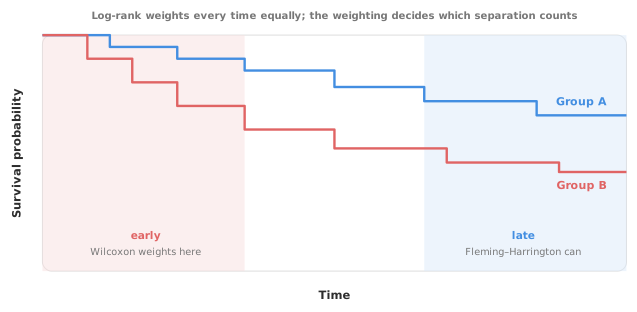
The choice of test is a decision about the clinical question, not a technicality, and it should be made before you see the data. Picking the test with the smallest p-value after the fact is like choosing a diagnostic cut-off on the same sample you then evaluate it on. Both practices produce results that look better than the data support.

Reading the result

A group-comparison test answers one question: is there a difference? What it does not tell you is how large the difference is, in which direction or whether it matters clinically. In a huge cohort, a significant log-rank test between two curves that barely separate reflects a difference that is real but trivial. A non-significant test on a small study may simply be underpowered.

Always read the test alongside the curves themselves and, where you need an effect size, a hazard ratio from a Cox model. The p-value is the beginning of the interpretation, not the end of it.

Common mistakes

Using a test that ignores censoring. A t-test or chi-square on survival times is wrong when observations are censored. The log-rank family is built to handle censoring.

Choosing the test after seeing the data. Running all four weightings and reporting the one that reaches significance inflates the false-positive rate. Choose the weighting from the clinical question, in advance.

Reading a p-value as an effect size. The test says whether the curves differ, not by how much. Pair it with the curves and a hazard ratio.

Treating “not significant” as “equivalent”. A non-significant comparison may be underpowered, so failing to detect a difference does not show that none exists.

Downloads

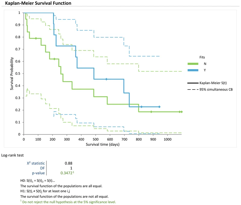
Download the Kaplan–Meier example workbook (.xlsx) — brain cancer survival in 30 patients, analysed by the yes/no Fits factor (19 patients against 11) and by tumour grade over three groups. Both analyses give mean survival restricted to [0, 1000] days and median survival with 95% confidence intervals, quartile survival times and a log-rank test. The Fits analysis adds a 95% simultaneous confidence band, and the tumour grade analysis a log [−log S(t)] vs log t plot. The workbook is ready to open in the Analyse-it trial.