
A log-rank test answers whether survival differs between groups. The test does not quantify the effect, adjust for other factors or handle a continuous predictor such as age.
Cox proportional hazards regression does all three. The hazard is the instantaneous rate of the event among those still at risk. The model treats the hazard as a baseline hazard multiplied by the combined effect of the covariates:
h(t | x) = h0(t) × exp(β1x1 + β2x2 + … + βpxp)
Here h0(t) is the baseline hazard, the event rate over time for a subject whose covariates are all zero. The exponential term scales that baseline up or down. Because the covariates enter multiplicatively, exponentiating a coefficient gives a hazard ratio: the factor by which the hazard is multiplied for a one-unit increase in that covariate.
Cox regression is described as semi-parametric because it leaves h0(t) completely unspecified. The omission is the model’s central trick, and it is worth understanding rather than accepting.
Fitting uses a partial likelihood. The method asks a narrow question at each time an event occurs. Given that exactly one subject in the risk set had the event at this instant, what is the probability it was the subject who actually did? The answer is that subject’s hazard divided by the total hazard across everyone still at risk. Every one of those hazards contains the same h0(t) factor, so it cancels from top and bottom. The baseline hazard drops out of the arithmetic entirely.
Multiply those probabilities across all the event times and you have the partial likelihood, which depends only on the coefficients. Maximising it estimates the covariate effects without ever committing to a survival distribution. The fit assumes no exponential, no Weibull and nothing about the shape of the underlying risk over time. That freedom is why Cox regression became the default for time-to-event data.
What the model does need is the data in the right shape. For each subject, the data must give a follow-up time, the covariate values and an indicator of whether that time ended in the event or in censoring. Where two or more events share a recorded time, a Cox fit needs a correction for ties, because the partial likelihood above assumes one event at a time. Efron’s method is the more accurate. Breslow’s is simpler, and is the default in several packages.
A hazard ratio is multiplicative and is read against 1. A ratio of 1 means the covariate makes no difference to the rate of the event. A ratio above 1 means the covariate raises the hazard: 1.07 per year of age means the event rate rises about 7% with each additional year. A ratio below 1 means it lowers the hazard, a protective effect.
The confidence interval is what makes the estimate usable. An interval lying entirely above or entirely below 1 is a significant effect. An interval that crosses 1 is not significant, however far the point estimate sits from it. The data are then compatible with the covariate raising the hazard, lowering it or doing nothing.
An interval that crosses 1 does not establish that there is no effect, only that the study could not detect one, and those are different findings. A hazard ratio of 1.9 with an interval from 0.8 to 4.5 is an imprecise estimate of something possibly substantial. A hazard ratio of 1.02 with an interval from 0.97 to 1.07 is good evidence that any effect is small. Both cross 1, and only the second supports a claim of no important effect. Read the width, not just whether the line was crossed.
Because hazard ratios multiply, they belong on a log scale, where a doubling and a halving sit the same distance from 1.
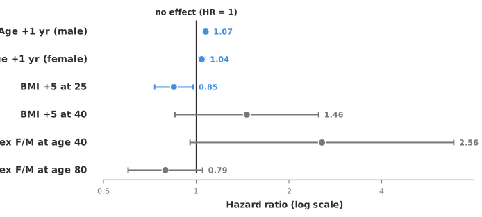
The model reports a coefficient for each term with its confidence interval and a test against zero on the log-hazard scale. The exponentiated coefficients are hazard ratios on the natural scale.
Alongside the individual terms is a likelihood-ratio test of the whole model against a null model. The test is the survival equivalent of an overall F-test, and it says whether the covariates together explain the survival pattern. In the worked example that whole-model test is decisive. The individual hazard ratios then locate the effect. Age and heart rate raise the hazard, and body-mass index and sex act in ways that depend on the rest of the model.
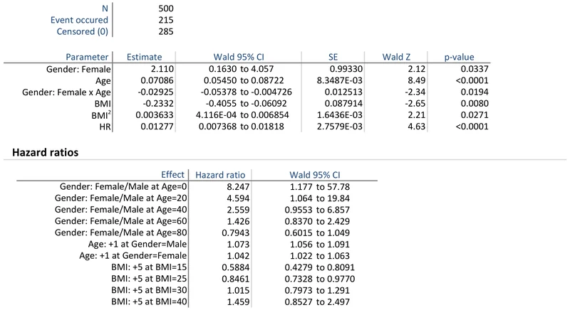
A common misreading is to quote one hazard ratio for a covariate when the model says the effect depends on another. The worked model includes a sex-by-age interaction, so no single hazard ratio for sex exists. The female-to-male ratio is 2.56 at age 40 and 0.79 at age 80. Neither interval excludes 1. What the model establishes is that the sex effect changes with age, not its size at any one age.
The model also carries a squared body-mass-index term. A five-unit rise in BMI from 25 to 30 is significantly protective (hazard ratio 0.85). The same rise from 40 to 45 points the other way (1.46), though that interval crosses 1. Neither ratio is a quirk to average away: together they show that the effect of BMI on the hazard changes across its range.
When a model contains interactions or non-linear terms, quote each hazard ratio at stated covariate values, exactly as the hazard-ratio table does. Here that means sex at a stated age, and a BMI change from a stated BMI. A single number for either covariate would misrepresent the model.
Everything above rests on one assumption in the name: the hazard ratio for a covariate is constant over time. The hazards for any two individuals stay in fixed proportion. When that holds, a single hazard ratio summarises the whole follow-up.
When the assumption fails, as with a treatment effect that fades or a risk that appears only late, the reported ratio is an average over follow-up. The weighting of that average depends on the censoring pattern. Such an average describes no particular moment, and it can mislead.
Check the assumption rather than assume it. Three approaches are standard, and they complement each other. A plot of Schoenfeld residuals against time should show no trend. A slope means the covariate’s effect is changing over follow-up, and the accompanying test puts a p-value on that change. A log-minus-log survival plot for a categorical covariate should show roughly parallel curves. And adding a covariate-by-time interaction to the model tests directly whether the effect moves with time.
Where the assumption fails, the restricted mean survival time (the area under the survival curve up to a fixed horizon) gives an effect measure that needs no proportionality. Use that when the assumption is in doubt.
Quoting one hazard ratio when the model has an interaction. If the effect depends on another covariate, the ratio must be evaluated at stated levels of it. A single number hides the interaction that the model was built to estimate.
Reading a hazard ratio as a risk ratio. A hazard ratio compares instantaneous rates, not cumulative probabilities. Over a long follow-up the two can diverge substantially.
Assuming proportional hazards rather than checking. When the assumption fails, the hazard ratio is a time-average that fits no single moment. Test it, and fall back on restricted mean survival time where it does not hold.
Treating a wide interval that crosses 1 as “no effect”. A non-significant covariate may be null or simply imprecisely estimated. The interval’s width tells you which.
Download the Cox proportional hazards example workbook (.xlsx) — the Worcester Heart Attack Study, 500 patients with 215 events. The model includes sex, age, their interaction, body-mass index as a quadratic and heart rate. The analysis gives parameter estimates with Wald 95% confidence intervals, hazard ratios at several ages and BMI values, and likelihood-ratio tests for the model and each term. The workbook is ready to open in the Analyse-it trial.
Analyse-it fits proportional hazards models on your own time-to-event data, inside Excel:
Every feature from all five editions for 15 days. Survival analysis is in the Medical and Ultimate editions, from US$ 340 a year. The same editions include Kaplan–Meier estimation and the group-comparison tests. Full detail in the survival and reliability reference guide.