
Cohen’s kappa (κ) measures how well two raters, or two methods, agree on a categorical result once the agreement expected by chance is removed. The obvious summary is the proportion of cases they agree on, but some of that agreement is free. If a condition is common, two raters who both lean towards “positive” will coincide often without either being any good. Raw agreement counts that luck as skill, and the rarer or commoner the condition, the more it misleads.
Kappa rescales observed agreement against chance agreement. Observed agreement, written po, is simply the proportion of cases the two raters classified the same way — the diagonal of the table divided by the total. The same quantity is sometimes called the percent agreement or overall percent agreement. The agreement expected by chance, pe, follows from the raters’ marginal rates: how often each rater uses each category. The marginal rates are read from the row and column totals of the table. Kappa is then:
κ = (po − pe) / (1 − pe)
The numerator is how much you beat chance. The denominator is how much you could have beaten it. κ = 1 is perfect agreement. κ = 0 is agreement no better than chance. Negative values mean the raters disagree more than chance would predict.
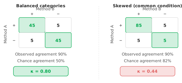
Take 100 samples where two raters agree on 45 positives and 45 negatives, and disagree on 10, five each way. Observed agreement is 0.90. Each rater called 50 positive and 50 negative, so chance agreement is (0.5 × 0.5) + (0.5 × 0.5) = 0.50. Kappa is (0.90 − 0.50) / (1 − 0.50) = 0.80. A kappa of 0.80 means 80% of the possible above-chance agreement has been achieved.
Plain kappa treats every disagreement as equally wrong, which is right for nominal categories and wasteful for ordered ones. If a grade can be 1, 2, 3 or 4, a 3-versus-4 split is a near miss and a 1-versus-4 split is a serious conflict. Those two errors should not count the same.
Weighted kappa assigns partial credit by distance from the diagonal. Linear weights penalise in proportion to how many categories apart the two calls are. Quadratic weights penalise the square of that distance, so near misses cost little and the penalty rises steeply with distance. State which weighting you used, because the two can give materially different numbers on the same table.
Which to choose depends on how the scale behaves. Linear weights suit a scale where each step is about as serious as the next. Quadratic weights suit one where large disagreements matter disproportionately. Quadratic weighting is the convention in much of the clinical and educational literature, and often the expected default. The quadratic form also has a useful property. On an ordered scale it is equivalent to the intraclass correlation coefficient computed on the category numbers, apart from a small-sample term (Fleiss and Cohen, 1973).
One question comes up often enough to answer directly. With only two categories, weighted kappa and unweighted kappa are the same number. Weighting adjusts the credit given to disagreements by how far apart they are. In a binary table every disagreement is exactly one category apart, so the weights have nothing left to distinguish. Weighting only changes the result once there are three or more ordered categories.
Kappa depends on the marginal totals, and that dependence has a well-known consequence. Keep observed agreement at 0.90 but skew the table: 85 samples both-positive, 5 both-negative, 10 split. Now each rater calls 90 positive and 10 negative. Chance agreement climbs to (0.9 × 0.9) + (0.1 × 0.1) = 0.82. Kappa collapses to (0.90 − 0.82) / (1 − 0.82) = 0.44.
Same 90% agreement, about half the kappa. The raters are no worse; only the base rate changed. When a condition is very common or very rare, chance agreement is already high, so there is little room left for kappa to reward.
Always read kappa next to the raw agreement and the marginal rates, never on its own. The output below reports all of them together for two qualitative methods.
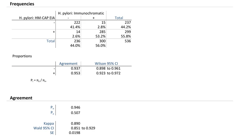
Report kappa with a confidence interval, because a single figure hides how much the estimate would move on a fresh sample. For an ordered scale, report weighted kappa and name the weights. Give the raw agreement and the marginal totals alongside, so a reader can see whether a low kappa reflects poor agreement or merely a skewed base rate.
The familiar interpretive bands come from Landis and Koch (1977):
| κ | Conventional label |
|---|---|
| < 0.00 | Poor — worse than chance |
| 0.00 – 0.20 | Slight |
| 0.21 – 0.40 | Fair |
| 0.41 – 0.60 | Moderate |
| 0.61 – 0.80 | Substantial |
| 0.81 – 1.00 | Almost perfect |
Use those labels with caution. Landis and Koch themselves called the divisions arbitrary, and none was derived from a clinical requirement. The bands also take no account of the prevalence effect, which is how the same 90% agreement can be labelled “substantial” on one table and “moderate” on another. What counts as adequate agreement depends on what the classification will be used for.
Download the CLSI EP12-A2 example workbook (.xlsx) — two qualitative methods compared, with observed and chance agreement, kappa, and its Wald confidence interval, ready to open in the Analyse-it trial.
The example workbook is downloading.
It opens in Excel on its own — the data and the finished results are both in it. Analyse-it is what lets you change the analysis and re-run it, try the same study on your own data, or work through it to see how the software handles it.
Every feature from all five editions for 15 days.
Reporting kappa without prevalence. A kappa of 0.44 can mean poor agreement, or excellent raw agreement on a lopsided sample. Publish the agreement and margins next to it.
Using unweighted kappa on an ordered scale. Grades and stages carry order. Unweighted kappa throws it away, treating a near miss as badly as a gross error. Weight it.
Using kappa alone to characterise a diagnostic test. The US Food and Drug Administration (FDA) discourages relying on kappa, or on overall percent agreement, on its own to describe diagnostic performance. Both can stay high while the test fails on one category. See performance studies for an IVD 510(k).
Leaning on the interpretive bands. “Substantial agreement” sounds definitive but rests on arbitrary cut-offs. Treat the label as shorthand, not evidence.
Ignoring the interval. Kappa from a small sample is unstable. A confidence interval that spans two of the interpretive bands is telling you not to over-read the point estimate.
Analyse-it reports kappa in its agreement analyses for binary and semi-quantitative results, inside Excel:
Every feature from all five editions for 15 days. Qualitative agreement is in the Medical, Method Validation and Ultimate editions, from US$ 340 a year. Validated against NIST and CLSI reference datasets. See PPA and NPA vs sensitivity and specificity for agreement without a gold standard, and the method comparison reference guide for the technical detail.