
A p-value and a confidence interval are computed from the same data and the same model. For a simple comparison you can derive one from the other. The two nonetheless lead readers to very different conclusions.
Report the estimate and its interval, not just the p-value. A mean difference of 0.3 mg/L with a 95% interval of 0.1 to 0.5 is a different finding from 0.3 with an interval of −0.4 to 1.0. The point estimate is the same, but the first establishes a positive difference and the second leaves the question open.
A p-value is the probability of observing data at least as extreme as yours, if the null hypothesis were true. That conditional clause is the key point. Almost every misinterpretation comes from dropping it.
A p-value is not the probability that the null hypothesis is true. Nor is it the probability that your result occurred by chance, or one minus the probability that the alternative is true. Its size is not a measure of effect size: p = 0.001 does not mean a bigger or more important effect than p = 0.04. A smaller p-value means the data are less compatible with the null. That compatibility depends on sample size at least as much as on the size of the effect.
With a large enough sample, a difference far too small to matter will produce a very small p-value. With a small sample, an important difference may not reach significance at all. The p-value confounds “how big” with “how much data”, and reports the mixture as a single number.
A 95% confidence interval is the range of values for the quantity that are compatible with your data. The method that constructs it is designed so that, over many repetitions, 95% of such intervals would contain the true value.
A confidence interval separates the two things the p-value confounds. Its position tells you how big the effect is. Its width tells you how well the study pinned it down. Both are on the scale of the measurement, so you can judge importance directly rather than through a probability.
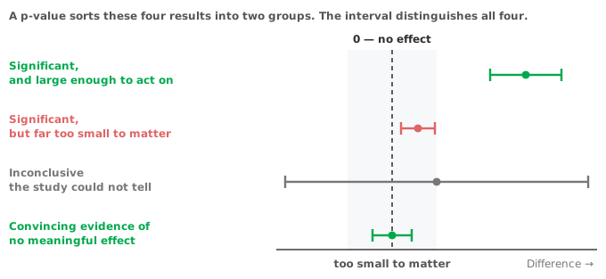
The third and fourth cases matter most. A p-value calls both “not significant”, yet they mean very different things. A wide interval crossing zero says the study could not tell. A narrow interval straddling zero, entirely inside the range of differences too small to care about, is positive evidence that any real effect is negligible. Reporting both as “no significant difference” throws away the distinction between ignorance and a genuine negative finding.
“Significant” is a technical term meaning “distinguishable from the null given this much data”. The technical term carries none of the everyday meaning of importance. The collision between the two is responsible for a great deal of over-claiming.
Deciding what would matter is a subject-matter judgement, made before the analysis and independent of it. In laboratory work it often already exists in written form: an allowable difference, a performance specification, a tolerance. A written specification makes the comparison concrete: does the confidence interval lie entirely inside the allowable limit? The same question underlies allowable total error and judging bias at a medical decision point, and it is a considerably better question than whether a p-value cleared 0.05.
Reading intervals this way also reframes what a “negative” result is. If you want to show two things are equivalent, a non-significant difference is not evidence of equivalence. You show equivalence by demonstrating that the whole confidence interval falls within the limits you would tolerate. For the usual 5% equivalence test, that is the 90% confidence interval.
Nothing changes in nature between p = 0.049 and p = 0.051. Treating the threshold as a cliff edge encourages two bad habits: dismissing results just above it, and stopping all further thought about results just below it.
Two related distortions are worth naming. Testing many things and reporting the significant ones inflates the error rate, which is why multiple comparison procedures exist. Collecting data until significance appears, then stopping, guarantees you will eventually reach it whether or not anything is there. Both are less tempting when the reported output is an interval, because an interval has no pass mark to aim at.
Strictly, the 95% refers to the procedure, not to your particular interval: over many repeated studies, 95% of intervals constructed this way would contain the true value. The 95% is not a probability that the true value lies in the particular interval you have.
For practical purposes, treating the interval as the range of values the data are consistent with is a sound working reading. That reading is far more useful than any reading of a p-value. Adopt two further habits. First, attend to the whole interval, including the ends. If the lower limit would still be an acceptable result and the upper limit would be alarming, the study has not settled the question. Second, remember that the interval reflects sampling variation only, and says nothing about bias, calibration error or a systematically unrepresentative sample. More data narrows the interval but does nothing to reduce any of those.
Download the compare-groups example workbook (.xlsx) — two independent groups reported with the mean difference and its confidence interval alongside the t-test, so you can see both presentations of the same result side by side.
The example workbook is downloading.
It opens in Excel on its own — the data and the finished results are both in it. Analyse-it is what lets you change the analysis and re-run it, try the same study on your own data, or work through it to see how the software handles it.
Every feature from all five editions for 15 days.
Reading p as the probability the null is true. It is the probability of data at least as extreme as yours, given the null, which is a different quantity.
Reading a small p as a large effect. It reflects sample size as much as effect size. The estimate tells you the size.
Reporting non-significant as no difference. Check whether the interval is narrow around zero or simply wide.
Treating 0.05 as a boundary in nature. It is a convention, and 0.049 and 0.051 say almost the same thing.
Deciding what counts as important after seeing the result. That judgement belongs before the analysis, and often already exists as a written specification.
Thinking a confidence interval covers all the uncertainty. It covers sampling variation. Bias and unrepresentative sampling sit outside it.
Analyse-it reports the estimate and its interval alongside the test wherever there is an effect to estimate, inside Excel:
Every feature from all five editions for 15 days. Hypothesis testing is part of the Standard edition, so it is in every Analyse-it edition, from US$ 155 a year. Validated against NIST Standard Reference Datasets. See choosing the right statistical test to work back to the analysis, or the study designs reference guide for the technical detail.