
“How many samples do I need?” has no single answer. The number depends on a question only you can settle: how small a difference would still matter enough that you would want to detect it? Fix that, and the arithmetic follows. Refuse to fix it, and no calculation is possible. Skipping that decision is how studies end up sized by convention, budget or what fitted on the plate.
Five quantities are bound together: the sample size, the difference you want to detect, the variability of the measurement and the two error rates. Fix any four and the fifth is determined.
The difference worth detecting. This is not the difference you hope or expect to find, but the smallest one that would change a decision. Setting that difference is a scientific judgement, not a statistical one, and it is the input that most often goes unexamined.
The variability. This is the standard deviation (SD) of the measurement within a group, taken from pilot data or historical records on comparable subjects. For groups of subjects, that SD includes between-subject variation as well as analytical imprecision. A precision study gives only the analytical part, which is enough only when the groups are reagent lots or instruments measuring aliquots of the same material. Everything downstream depends on the SD, which is usually the least certain of the inputs.
The significance level α, the false-positive rate, is conventionally 5%.
The power, the chance of detecting the difference if it is really there, is conventionally 80%. An 80% power means accepting a one-in-five chance of missing a real effect you have decided you care about. For high-stakes work, 90% is a better choice.
The difference and the variability enter only as their ratio, the standardised effect size: difference divided by standard deviation. The ratio is convenient: one table covers every measurement scale.
Approximate subjects per group for a two-sided comparison of two independent means at α = 0.05:
| Standardised effect (difference ÷ SD) | 80% power | 90% power |
|---|---|---|
| 0.2 — a fifth of a standard deviation | 394 | 527 |
| 0.5 — half a standard deviation | 64 | 86 |
| 0.8 | 26 | 34 |
| 1.0 — a full standard deviation | 17 | 23 |
To use it: if you want to detect a difference of 4 units and the within-group SD is 8 units, the standardised effect is 0.5. Plan for about 64 per group at 80% power. The table gives planning figures only. Add a margin for dropouts, and remember that the figures are only as reliable as the SD behind them.
What matters most in that table is its shape. Halving the effect you want to detect multiplies the required sample by roughly four. Going from 0.5 to 0.2, a difference that can still matter in practice, takes you from 64 per group to nearly 400.
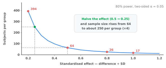
Two practical consequences follow. First, reducing analytical variability shrinks the SD, which buys the same statistical benefit as a larger sample, often more cheaply. Better technique, averaged replicate measurements or a more precise method all count, although none of them reduces the variation between subjects. Second, a study too small to detect the difference you care about risks more than an inconclusive result. A non-significant result from such a study is easily read as evidence of no difference.
For a paired design, the variability that matters is not the variation between subjects but the variation in the within-subject difference, which is usually far smaller. The same table applies, with the standardised effect computed against the SD of the differences.
When subjects differ substantially but respond consistently, pairing can reduce the required sample several-fold. Pairing is often the most effective design change available, and it costs only the ability to measure each unit twice. See Student’s, Welch’s or paired for what pairing does to the analysis.
Two other design points matter. Equal group sizes are the most efficient allocation for a fixed total. The loss from moderate imbalance is small, but severe imbalance is governed by the smaller group. A split of 180 versus 20 gives the same precision as 36 per group: 72 subjects in total, not 200. If the outcome is a proportion rather than a mean, the arithmetic differs. Proportions near 0.5 need the most subjects for a given difference. For the diagnostic-accuracy case, where each arm is sized separately, see how many samples for a diagnostic accuracy study.
After a non-significant result, it is tempting to compute the power the study had. Do not bother. Power computed from the observed effect is a deterministic function of the p-value, so it carries no information the p-value did not already give you. Observed power is always below about 50% when the result was non-significant, which makes reporting it circular.
The informative thing to report is the confidence interval on the difference. An interval from −0.5 to +0.7 units, against a difference of 3 units that would have mattered, is genuine evidence that any real effect is small. An interval from −8 to +15 says the study could not tell, which is a quite different statement. Either way, the interval is what you should report. Confidence intervals and p-values takes this further.
Prospective power calculations, on the other hand, are worth doing properly and recording before the data exist. The record also fixes the primary comparison before the data can influence it.
With three or more groups, size the study on the specific comparison that matters most rather than on the overall F-test. Remember that the multiple comparison procedure widens intervals. A design powered for a single unadjusted comparison will be underpowered once the adjustment is applied. Narrowing the family of comparisons is, once again, the cheapest way to recover the lost power.
The same applies to multiple endpoints. A study with six outcome measures, each tested at 5%, has about a 26% chance of at least one spurious finding if the outcomes are independent. Declaring one primary endpoint in advance is the usual answer.
Sizing on the effect you expect rather than the smallest one that matters. The first is optimism; the second is the design input.
Computing post-hoc power. It restates the p-value. Report the confidence interval instead.
Using an SD from a source that does not resemble your study. The required sample scales with its square. A published SD from a different population or method can be badly wrong.
Reading non-significant from a small study as no difference. A non-significant result from a small study is absence of evidence, and its wide interval says so plainly.
Sizing for an unadjusted comparison, then adjusting. The multiple comparison procedure consumes the power you planned.
Forgetting attrition. The sample size is what you need at analysis, not at enrolment.
Plan the study so the interval lands where you need it; Analyse-it then reports the estimate that shows whether it did, inside Excel:
Every feature from all five editions for 15 days. Hypothesis testing is part of the Standard edition, so it is in every Analyse-it edition, from US$ 155 a year. Validated against NIST Standard Reference Datasets. Where the comparison is between reagent lots or instruments on shared material, the SD comes from a precision study, covered by Method Validation.