
A sensitivity of 90% sounds settled until you see it came from 18 of 20 diseased subjects. The 95% confidence interval runs down to around 70%. The point estimate is not the finding. The interval is. So the design question is not “how many samples give me 90%?” but “how many samples give me 90% ± something I can live with?”
The width of a proportion’s interval scales with the square root of p(1 − p) / n, and two consequences follow. Precision improves only with the square root of the sample size, so halving the interval takes roughly four times the subjects. And because p(1 − p) is largest at 0.5, proportions near 0.5 need the most subjects. Proportions near 1 need fewer, which is fortunate, because sensitivity and specificity are usually high.
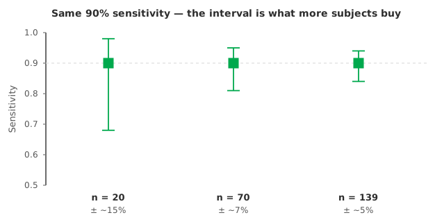
Sizing the two arms separately is the step many plans miss. Sensitivity is estimated only from the diseased subjects and specificity only from the non-diseased, so the two arms are separate sample-size problems. The width of each interval is governed by the count in that arm, not by the total. For a rare condition sampled consecutively, the non-diseased arm fills quickly while the diseased arm fills slowly, so the diseased arm usually limits the study. Sizing a study to compare two tests against each other is a different calculation again, covered below.
Approximate number of subjects in each arm for a two-sided 95% interval of the stated half-width, at the expected proportion:
| Expected sensitivity (or specificity) | ±10% | ±7% | ±5% |
|---|---|---|---|
| 80% | 62 | 126 | 246 |
| 90% | 35 | 71 | 139 |
| 95% | — | 38 | 73 |
Read it as: to pin a sensitivity you expect near 90% to within ±5%, plan for about 139 diseased subjects. Plan separately for enough non-diseased subjects to pin specificity to the width you need. The table gives planning figures from the normal approximation. The interval you finally report should use a method that behaves near the boundary, such as Wilson. The 95% row has no ±10% figure, because near 100% the interval is lopsided and the approximation fails. With 19 subjects at 95%, for example, the Wilson lower limit is about 75%, not 85%. Plan so that the lower confidence limit, not the point estimate, meets your requirement.
The sample size depends on three things when the endpoint is the area under the ROC curve rather than a single operating point. The three are the AUC you expect, the width you want and the allocation between diseased and non-diseased groups. A higher expected AUC needs fewer subjects for the same precision. If the study exists to show one test beats another, you are sizing for the difference in AUC. A paired design, with both tests run on the same subjects, needs far fewer than two independent groups, because pairing removes between-subject variation from the comparison.
Enrolling consecutive patients preserves the true prevalence and the natural case mix, which protects you from spectrum bias. But for a rare condition it leaves the diseased arm short. Enriching the diseased group fixes the count but distorts prevalence and, if the extra cases come from a different setting, the case mix too. Predictive values from an enriched study are meaningless unless you re-anchor them to a real prevalence (or report likelihood ratios instead). Decide which you are doing before enrolment, not after.
Sizing on the total, not the arms. Two hundred subjects with eight diseased give a precise specificity and a useless sensitivity. Count the arms separately.
Planning for the estimate, not the interval. “We need to show 90%” is not a sample size. “We need 90% to within ±5%” is.
Enriching, then quoting a predictive value. Predictive values depend on prevalence. Enrichment has thrown the prevalence away. Report likelihood ratios, or re-anchor to a real prevalence.
Sizing without the submission in mind. Where the study supports a regulatory claim, the reporting expectations shape the design as much as the target precision does. See performance studies for an IVD 510(k).
Forgetting the spectrum. Easy cases inflate both sensitivity and specificity. A study sized perfectly on clear-cut subjects still misleads about performance in the ambiguous middle where the test is actually used.
Plan the study so the intervals land where you need them; Analyse-it then shows the precision you actually got, inside Excel:
Every feature from all five editions for 15 days. Diagnostic accuracy is in the Medical, Method Validation and Ultimate editions, from US$ 340 a year. Validated against NIST and CLSI reference datasets. See how many samples for a method comparison for the quantitative counterpart.