
Every t-test compares a difference against the uncertainty in that difference. What separates the variants is what they assume about where the numbers came from. One choice, paired or independent, is fixed entirely by your study design, and getting it wrong either wastes the data or invalidates the analysis. The other choice is a judgement about variances, and the conventional answer to it is the wrong one.
One confusion is worth clearing up before anything else, because it turns up constantly: Welch’s is not a third option alongside paired and unpaired. Welch’s is a variant of the unpaired test. The design decides paired against unpaired first, and only then, if the design is unpaired, does the variance question decide Student’s against Welch’s. There is no such thing as a paired Welch’s t-test, because the paired test works on one set of differences and so has only one variance to estimate.
| Test | Design | Assumes equal variances |
|---|---|---|
| Paired t-test | Same subject measured twice | Not applicable — one set of differences |
| Student’s t-test (unpaired) | Different subjects in each group | Yes — pools them into one estimate |
| Welch’s t-test (unpaired) | Different subjects in each group | No — uses each group’s own variance |
Neither Student’s nor Welch’s is a non-parametric test. Both assume approximate normality; what Welch’s drops is the equal-variance assumption, not the normality one.
Independent samples, also called unpaired, means different subjects in each group. Think of a treated group and a control group, or samples from two suppliers. Paired means the same subject, specimen or unit measured twice: before and after, two methods on one sample, matched case-control pairs.
A paired test does not compare two groups at all. The test computes the difference within each pair and asks whether those differences average to something other than zero. That single change is why pairing is so effective: differences between subjects, often the largest source of variation in the whole study, cancel out of the comparison completely.
The gain can be dramatic. If subjects vary widely but each responds consistently, a paired design can detect with twenty pairs what an independent design would need hundreds of subjects to see. Analysing paired data as independent throws all of that away and will often miss a real effect. Analysing independent data as paired is not just wasteful but wrong, since there are no genuine pairs to difference.
For independent samples, Student’s t-test assumes both groups have the same variance and pools them into a single estimate of spread. Welch’s t-test does not: it uses each group’s own variance and adjusts the degrees of freedom accordingly. Use Welch’s by default. Where the variances really are equal, Welch’s loses almost nothing. Where they are not, Student’s test can be badly wrong, especially when the group sizes are unequal too. The test’s real error rate can then sit well away from the 5% it claims.
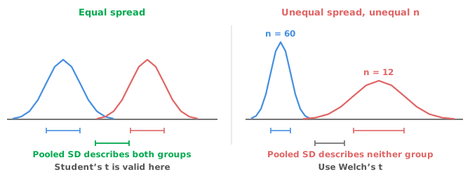
The preliminary variance test is itself a problem, not just an inconvenience. Choosing which test to run based on the outcome of another test on the same data makes the properties of the final result something other than advertised. The same objection applies to screening with a normality test, covered in testing normality. Variance tests are worth running to understand your data, but not to select your t-test.
The t-test makes three assumptions, listed here in descending order of importance.
Independence of observations. Independence is essential, and no choice of t-test can repair its absence afterwards. Three measurements on each of ten subjects are not thirty independent observations. No variant of the t-test will notice if you pretend otherwise.
Equal variances, for Student’s only. This is what Welch’s exists to sidestep.
Approximate normality. Normality is the least demanding of the three, and what matters is the sampling distribution of the mean rather than the raw data. With a few dozen observations per group the central limit theorem does most of the work and moderate skew is tolerable. At small n, heavy tails and outliers still cause problems, because the mean and standard deviation are both sensitive to extreme values.
For a paired test, the assumption applies to the differences, not to either set of original measurements. That distinction matters, because differences are often well behaved even when the underlying values are skewed.
When normality is genuinely doubtful and the sample is small, the Wilcoxon-Mann-Whitney test replaces the independent-samples t-test. The Wilcoxon signed-ranks test replaces the paired one. Both work on ranks and make no assumption of normality. The signed-ranks test does assume the differences are roughly symmetric. The sign test goes further still, using only the direction of each difference, which makes it robust to any distributional shape and correspondingly blunt.
Rank tests cost less power than people expect, but they answer a subtly different question, about distributions and typical values rather than means. Understand that difference before you switch. Non-parametric tests covers the trade.
A t-test tells you whether a difference is distinguishable from noise. What it does not tell you is how big the difference is, which is usually what you actually need. The mean difference with a confidence interval should be the headline. The mean difference is on the scale of the measurement, so it is directly interpretable. The interval’s width tells you how well the study pinned the answer down.
A standardised effect size expresses the difference in standard deviations. Cohen’s d and Hedges’ g are the usual ones. Sources define them differently, by the variance estimate used and whether a small-sample correction is applied. Standardised effects are useful when comparing across studies or when the raw units mean nothing to the reader. For rank-based analyses the Hodges-Lehmann location shift is the natural companion estimate, and it comes with a confidence interval too.
The two failure modes here mirror each other, and both are common. One is a significant result that is far too small to matter, found only because the sample was large. The other is a non-significant result reported as “no difference” when the interval runs from −8 to +15 and the study was simply too small to say anything. See confidence intervals and p-values.
If there are three or more groups, do not run t-tests on every pair. Three groups give three comparisons, six give fifteen, and the family-wise error rate climbs fast. One-way ANOVA is the right starting point. Welch’s ANOVA is the unequal-variance version, following the same reasoning as above. Follow with a multiple comparison procedure matched to the comparisons you need.
Download the independent-samples example workbook (.xlsx) — calcium supplementation and blood pressure in two groups, with box plots, a Fisher F test for the variance ratio and Student’s t-test. The example follows the variance-screening route this article advises against, so rerun it with Welch’s t-test and compare the results. The paired example covers body fat in 28 people before and after an exercise programme, with the Hodges-Lehmann shift, its confidence interval and the Wilcoxon signed-ranks test.
The example workbook is downloading.
It opens in Excel on its own — the data and the finished results are both in it. Analyse-it is what lets you change the analysis and re-run it, try the same study on your own data, or work through it to see how the software handles it.
Every feature from all five editions for 15 days.
Using an independent-samples test on paired data. This is the most expensive error here. Pairing removes between-subject variation, and ignoring it usually costs power and often the result.
Testing variances to decide which t-test to use. Use Welch’s by default and skip the screening step entirely.
Reporting only the p-value. The mean difference and its interval are the finding. The p-value is one thing you can read off them.
Reading non-significant as no difference. A wide interval means the study could not tell, which is not the same as an answer.
Running every pairwise t-test with three or more groups. Use ANOVA and a multiple comparison procedure.
Checking normality of the raw values in a paired design. It is the within-pair differences that need to be well behaved.
Analyse-it runs the test and reports the estimate you should be quoting, inside Excel:
Every feature from all five editions for 15 days. Hypothesis testing is part of the Standard edition, so it is in every Analyse-it edition, from US$ 155 a year. Validated against NIST Standard Reference Datasets.