
A parametric test assumes the data come from a distribution of a particular family, usually normal, and works with its parameters: the mean and standard deviation. A non-parametric test makes no such assumption about shape. Most of the ones in routine use achieve that by throwing away the values and keeping only their order.
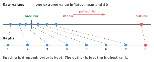
Replace every observation by its rank in the combined sample — smallest is 1, next is 2, and so on — and then work with the ranks. Ranks are always 1, 2, 3… whatever the original numbers were. The null distribution of the test statistic can therefore be worked out exactly, without knowing anything about the distribution the data came from.
Two properties follow immediately. The test is robust to outliers: the most extreme value in the dataset becomes simply the highest rank, no matter how far out it sits. And it is invariant to monotonic transformation: taking logarithms changes no rank, so the test gives the same answer on the log scale as on the original one. That invariance is a considerable convenience when the right scale is uncertain. The Wilcoxon signed-ranks test is the exception, because it ranks the paired differences, and taking logarithms changes their relative sizes.
The pairings are direct. The Wilcoxon-Mann-Whitney test replaces the independent-samples t-test. The Wilcoxon signed-ranks test replaces the paired t-test, and the sign test is the still more robust option that uses only the direction of each difference. Kruskal-Wallis replaces one-way ANOVA, and Friedman replaces the within-subjects version. Spearman’s rs and Kendall’s τ replace Pearson correlation, as covered in Pearson, Spearman or Kendall.
Follow-up comparisons exist too, and are just as necessary here as anywhere. Alongside a Kruskal-Wallis test, the Steel-Dwass-Critchlow-Fligner procedure compares all pairs and Steel’s procedure compares against a control. Both control the family-wise error rate, as described in choosing a multiple comparison procedure.
The persistent belief is that non-parametric tests are much less powerful. Under the conditions where the parametric test is exactly right (genuinely normal data), the Wilcoxon-Mann-Whitney test retains about 95% of the efficiency of the t-test. In practical terms the rank test needs roughly one extra subject in twenty to reach the same power, which is a small price.
When the data are not normal, the comparison often reverses, and even in the worst case the rank test keeps about 86% of the t-test’s efficiency. For heavy-tailed distributions, or data with occasional extreme values, the rank test can be substantially more powerful than the t-test. The reason is that the t-test’s standard deviation is inflated by the very observations the rank test neutralises.
The real trade, then, is not power but interpretation.
Rank tests are not assumption-free: they drop the assumption about shape and keep the others. Independence still matters exactly as much as before, and no rank test will detect or forgive clustered observations.
What the test compares depends on an assumption that is easy to overlook. Wilcoxon-Mann-Whitney is properly a test of whether a value from one group is more likely than not to exceed a value from the other. The test compares medians only under the additional assumption that the two distributions have the same shape and differ by a shift. If one group is far more spread out than the other, the test can return a significant result while the medians are identical. The distributions then differ, but not by a shift.
The signed-ranks test assumes symmetry. The Wilcoxon signed-ranks test assumes the paired differences are symmetric about their median. Where the differences are clearly skewed, the sign test is safer.
Ties reduce the information. Heavily tied data, from coarse scales or many repeated values, weaken rank tests, and Kendall’s τ handles ties more gracefully than Spearman does.
Very small samples may never reach significance. With three observations per group, no arrangement of ranks produces a two-sided p below 0.05. The test is not failing; there is simply not enough ordering information in six numbers.
The most common complaint about non-parametric tests is that they give a p-value and nothing you can quote as an effect. The complaint describes a habit rather than a limitation.
The Hodges-Lehmann location shift is the natural estimate, on the original measurement scale. For independent samples it is the median of all pairwise differences between the groups, with a Moses confidence interval. For paired data it is the median of all pairwise averages of the differences, with a Tukey interval. The Hodges-Lehmann shift is to the rank tests what the mean difference is to the t-test, and it should be reported the same way. A median difference with a Thompson-Savur interval is the alternative when the median itself is the quantity of interest.
Ordinal data. Ordinal data are the clearest case, and not really a choice. If the spacing between categories is not meaningful, the mean is not a quantity and only rank methods apply.
Small samples with visible skew or outliers. Small n is where non-normality actually costs you, since the central limit theorem is not yet helping.
Data with genuine extreme values you cannot justify removing. Robustness by design beats a judgement call about deletion.
When the median is the more meaningful summary. For strongly skewed quantities, such as times to event, costs or concentrations, the median often describes the typical case better than the mean does.
The case against arises when the mean is the quantity that matters, such as a total yield or an average cost per unit. A test about ranks then answers a different question. The t-test, which tolerates non-normality well in larger samples, or a bootstrap interval for the mean will serve better. Do not choose between them by running a normality test first; the reasons are in testing normality and what to do when it fails.
Download the paired comparison example workbook (.xlsx) — body fat in 28 people before and after an exercise programme, with the Hodges-Lehmann shift, its confidence interval and the Wilcoxon signed-ranks test, ready to open in the Analyse-it trial.
The example workbook is downloading.
It opens in Excel on its own — the data and the finished results are both in it. Analyse-it is what lets you change the analysis and re-run it, try the same study on your own data, or work through it to see how the software handles it.
Every feature from all five editions for 15 days.
Believing they assume nothing. Independence still applies, and interpreting the result as a difference in medians requires similar distribution shapes.
Avoiding them because of a supposed power penalty. The loss is about 5% in efficiency under ideal normality, and the rank test is often more powerful otherwise.
Choosing one after a normality test. Conditioning the analysis on a preliminary test distorts the properties of whichever you run.
Reporting only the p-value. The Hodges-Lehmann shift with its interval is an effect estimate on the original scale. Quote it.
Using them on tiny samples and reading non-significance as no effect. With three per group, significance is unreachable whatever the data show.
Using them to fix non-independence. Clustered or repeated observations need a design-level answer, not a different test.
Analyse-it runs them with the estimate attached, not just the p-value, inside Excel:
Every feature from all five editions for 15 days. Hypothesis testing is part of the Standard edition, so it is in every Analyse-it edition, from US$ 155 a year. Validated against NIST Standard Reference Datasets.