
The short answer first, for anyone who came here to pick a test. Shapiro-Wilk is the default test for normality and the most powerful of the general ones against most alternatives. Anderson-Darling is the better choice when the tails are what matter to you. Kolmogorov-Smirnov is the weakest of the three and is mainly of historical interest. In each case a small p-value says the data depart from normal. A large p-value says the test could not detect a departure, which is not the same as showing there is none.
The longer answer is that the test is rarely the thing you should act on. A normal Q-Q plot tells you more, because a test only ever says no, while the plot tells you how the data depart. The how is what decides your response.
“Is my data normal?” is asked constantly, and it is almost never the right question. No real measurement is exactly normal. Normality is a mathematical idealisation, and with enough data every dataset departs from it detectably. The useful question is different: is it close enough that the procedure I want to run will behave properly? The answer depends on the procedure, the sample size and the kind of departure. A normality test addresses none of the three.
A normality test gets more powerful as your sample grows, and that is the problem. With a large sample, the test detects departures far too small to matter. Two thousand observations with a mild skew will fail Shapiro-Wilk decisively. At that sample size the t-test you were about to run is essentially immune to skew that mild. The central limit theorem has long since taken care of the sampling distribution of the mean.
With a small sample, the test has little power, so it passes many clearly skewed distributions. A small sample is where non-normality does the most damage. The central limit theorem does not protect the mean of a small sample.
The test is most likely to raise the alarm when you can safely ignore the problem, and least likely to raise it when you cannot. The test’s sensitivity runs backwards to the risk, and reliably so.
A normal Q-Q plot orders your observations and plots them against the values you would expect if the distribution were normal. Points close to a straight line mean the data are consistent with a normal distribution. The way they leave the line names the departure. The patterns below have the data on the vertical axis. Analyse-it’s Distribution and Compare Groups plots put the data on the horizontal axis, which mirrors each pattern about the line. Right skew then bends below the line at both ends.
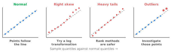
A confidence band around the reference line shows how much wander is ordinary at your sample size. A Lilliefors band on the Q-Q plot, or a Kolmogorov-Smirnov band on a CDF plot, gives that context. It stops small samples looking alarming. A histogram with a normal curve overlaid is a useful second look. The impression it gives depends heavily on the bin width, so treat it as a supporting view rather than the decisive one.
Anderson-Darling gives extra weight to the tails of the distribution, which is what makes it the better choice when the tails are what matter to you. Beyond that choice, the more useful question is what the tests are for.
Where they earn their place is as documentation rather than decision. If a protocol or an assessor requires evidence that the assumption was examined, a test result is an acceptable record. Reference interval work is the clearest case. Choosing a reference interval method turns on distributional shape in a way most procedures do not, because the estimates live in the tails. The same is true of process capability, where the defect rate is computed from a tail area and normality matters directly rather than incidentally.
Procedures that depend on a tail care a great deal about normality, and procedures about means care much less.
Robust, given a reasonable sample. The t-test, ANOVA and regression assume normality of the residuals. Their conclusions about means hold up well under moderate departures once you have a few dozen observations per group. Unequal variances are a bigger threat than mild non-normality, and heavy tails often matter more than skew because they inflate the standard deviation.
Genuinely sensitive. Anything that depends on a tail: reference limits, capability indices and their PPM defect rates, detection limits, prediction intervals for individual future values. Here the whole answer is a property of the tail, so getting the shape wrong changes the answer directly.
One recurring confusion is worth naming. Regression and ANOVA assume the residuals are normal, not the response and not the predictors. The check belongs after fitting, in the residual diagnostics, not before it on the raw data.
When normality fails, you have four options, roughly in order of preference.
Find out why. A bimodal distribution usually means two populations mixed together: two instruments, two operators, two lots. Splitting them is a better analysis than any transformation. A long right tail with a hard floor at zero is the natural shape of a concentration, not a defect. Non-normality is often information about the process, not a nuisance to remove.
Transform. A logarithmic transformation handles right skew and multiplicative variation, which between them cover most of what you meet in laboratory data. Box-Cox and other power transformations generalise the logarithm. The catch is interpretation. The analysis now concerns the transformed scale. Back-transforming a mean difference gives you a ratio of geometric means rather than a difference of arithmetic ones. A ratio is often perfectly reasonable, but it needs to be stated rather than glossed over.
Use a rank-based method. Wilcoxon-Mann-Whitney, Kruskal-Wallis, Spearman and the rest drop the normality assumption. Rank methods cost surprisingly little power when the data are normal after all, but they answer a slightly different question, about typical values rather than means. See non-parametric tests.
Use a method built for the shape. For a tail-dependent quantity, such a method is more accurate than forcing the data towards a bell curve. A non-parametric interval, a bootstrap and an explicitly non-normal model are the usual choices. Where outliers rather than shape are the issue, screening and handling them properly is a separate job from transforming.
Download the distribution example workbook (.xlsx) — Newcomb’s 64 measurements of the speed of light, ready to open in the Analyse-it trial. The workbook gives descriptive statistics, a histogram, a box plot, a normal Q-Q plot with a confidence band and the Shapiro-Wilk test.
The example workbook is downloading.
It opens in Excel on its own — the data and the finished results are both in it. Analyse-it is what lets you change the analysis and re-run it, try the same study on your own data, or work through it to see how the software handles it.
Every feature from all five editions for 15 days.
Testing normality to choose between a parametric and a non-parametric test. Conditioning one test on another distorts the properties of whichever you end up running. Decide from the design and the plot instead.
Rejecting normality on a large sample. At n = 5000 the test detects departures that would not have troubled your analysis in the slightest.
Accepting normality on a small sample. Passing the test at n = 15 is weak evidence of anything; the test simply cannot see much.
Testing the response instead of the residuals. Regression and ANOVA assume normal residuals. A skewed response with a well-behaved model is not a problem.
Transforming without saying so. The results are on the transformed scale, and a back-transformed mean on the log scale is a geometric mean. Report which scale you are on.
Treating non-normality as a nuisance to be removed. Bimodality and skew often carry the most interesting information in the dataset.
Analyse-it shows you which departure you have, not just whether there is one, in Distribution:
Every feature from all five editions for 15 days. Descriptive statistics are part of the Standard edition, so they are in every Analyse-it edition, from US$ 155 a year. Validated against NIST Standard Reference Datasets. See choosing the right statistical test for where the assumption fits in.