
Common factor analysis estimates a small number of unobserved variables, called factors, that account for the correlations among the variables you did measure. The factors are the constructs you believe exist but cannot observe directly: a patient’s anxiety, an instrument’s underlying drift, a respondent’s satisfaction.
Factor analysis starts from an explicit model of how the data arise. The model says each measured variable is driven partly by factors shared with the other variables, and partly by something belonging to that variable alone. Everything else follows from taking that split seriously.
The common factor model writes each observed variable as a weighted sum of the common factors, plus a term unique to that variable. The weights are the loadings. A loading is the strength of the link between one variable and one factor, and on standardised data it reads much like a correlation.
The unique term is the whole point. The variance of each variable divides in two. The part explained by the common factors is its communality, and the remainder is its uniqueness, a mix of genuine specific variance and measurement error. A variable with a communality of 0.7 shares 70% of its variance with the rest of the set and keeps 30% to itself.
Because the model separates those two pieces, factor analysis explains the correlations between variables rather than the total variance in them. The split is the substantive difference from principal component analysis, which re-expresses total variance with no model behind it and no notion of a unique part.
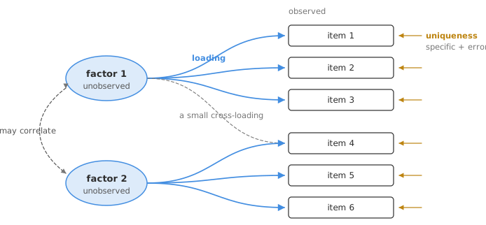
Extraction is the step that finds loadings consistent with the observed correlation matrix. Several methods exist, and the two in common use answer slightly different questions.
Maximum likelihood treats the model as a statistical one and finds the loadings that make the observed correlations most probable. The payoff is inference: standard errors for the loadings, and a goodness-of-fit test for whether a given number of factors reproduces the correlation matrix adequately. The cost is an assumption of multivariate normality, and a fit test that grows harsh as the sample grows, in the way any significance test does.
Principal axis factoring makes no distributional assumption and simply iterates on the communalities. The method gives no fit test, which is exactly why some people prefer it: no test to over-read.
Extraction produces one mathematically valid answer, not the answer. Any rotation of the factor solution fits the data equally well, which is what rotation exploits.
The number of factors is a judgement, and the usual mechanical rules are weaker than their popularity suggests. Take evidence from several places and expect them to disagree.
A scree plot shows the eigenvalues in order, and the elbow marks where additional factors stop explaining much. Reading an elbow is subjective, and on real data there is often more than one.
The eigenvalue greater than one rule is the most common and the least defensible. The rule was derived for the eigenvalues of the full correlation matrix, which belong to principal components. Factor analysis works on the reduced matrix, and there the rule systematically keeps too many factors.
Parallel analysis compares each eigenvalue against what random data of the same size would produce, and keeps a factor only where the real value exceeds the random one. In simulation studies this method performs better than either rule above.
Interpretability is the decision rule that matters most. A factor you cannot name, because its variables share nothing beyond a statistical association, is not a construct. Where a maximum likelihood extraction was used, the fit test adds one more piece of evidence. A solution that fails it may need more factors, although in a large sample a trivial misfit will also fail. Passing it is not on its own a reason to stop.
Rotation redistributes the loadings across factors without changing how well the model fits. The goal is simple structure: each variable loading strongly on one factor and weakly on the rest, so the factors can be named.
Orthogonal rotations, Varimax being the common one, keep the factors uncorrelated. The solution is tidy and each factor’s contribution is separable, which is convenient when the factors will be used as inputs to something else.
Oblique rotations, such as Oblimin and Promax, allow the factors to correlate. Real constructs usually do correlate, so an oblique rotation is often the more honest choice, and it reports the correlations between factors as part of the output.
One consequence is often missed. After an oblique rotation there are two matrices, not one. The pattern matrix holds the unique contribution of each factor to each variable, and is what you interpret. The structure matrix holds the plain correlations, which include the shared part. Quoting one and calling it the other misstates the loadings, often substantially.
State the extraction method, the rotation and the number of factors with the reasoning that settled it. Give the loadings, the communalities and, for an oblique rotation, the factor correlations. Say how large a loading had to be before you treated it as meaningful, and fix that threshold before you look.
Sample size belongs in the report as well. Rules of thumb are common and crude. The useful version is a statement about communalities rather than a count. Solutions with high communalities and several strong loadings per factor stabilise at far smaller samples than solutions with weak ones.
Where the factors will be used as a scale, report an internal-consistency estimate such as Cronbach’s alpha alongside them. Alpha answers a different question from the factor solution, and a set of items can load cleanly on one factor and still make an unreliable scale.
Download the multivariate example workbook (.xlsx) — a common factor analysis of 12 neighbourhood liveability measures, reporting uniqueness, communality and loadings, alongside a principal component analysis of the same data. The workbook is ready to open in the Analyse-it trial.
Running PCA and calling it factor analysis. The two answer different questions, and the software menus sit next to each other. If you want to estimate latent constructs, the method has to model unique variance. See principal component analysis explained for the other side of the distinction.
Keeping every factor with an eigenvalue above one. Applied to the full correlation matrix, as it usually is, the rule over-extracts factors. Use a scree plot and parallel analysis, and require that each retained factor can be named.
Interpreting the structure matrix after an oblique rotation. Interpret the pattern matrix. Report both if you like, but say which is which.
Naming a factor from its two largest loadings. A name has to account for every variable loading on the factor, including the ones that do not fit the story. A factor with an awkward member is telling you something.
Treating a factor solution as confirmed. Exploratory factor analysis generates a structure from the data. Confirming it needs a second, independent sample, and a solution that has never met one is a hypothesis.
Factoring variables that are not conceptually related. The method will always return factors. Feed it an arbitrary set of measurements and it returns arbitrary factors.
Analyse-it performs common factor analysis on your own item data, inside Excel:
Every feature from all five editions for 15 days. Factor analysis is part of the Standard edition, so it is in every Analyse-it edition, from US$ 155 a year. See Pearson, Spearman or Kendall for the correlations the method starts from, and the factor analysis reference guide for the technical detail.