
Plenty of outcomes are binary: the sample is positive or negative, the unit passes or fails, the patient responds or does not. Fitting a straight line to a 0/1 response causes two problems. The line keeps going, so it can predict probabilities greater than 1 at one end and less than 0 at the other. And the residuals cannot be normal, because the response takes only two values.
Logistic regression models the probability of the outcome instead, through a curve that approaches 0 and 1 without reaching either. The model is fitted by maximum likelihood rather than least squares. The result is a model that behaves sensibly across the whole range of the predictor.
The odds of an event are its probability divided by the probability of it not happening. A probability of 0.8 is odds of 4: four times as likely to happen as not.
Probabilities are bounded by 0 and 1, and odds run from 0 to infinity. The logarithm of the odds runs from minus infinity to plus infinity, which is the unbounded scale a linear model needs.
So logistic regression models the log-odds as a linear function of the predictors. The log-odds is called the logit, and the model is written:
logit(p) = ln( p / (1 − p) ) = β0 + β1x1 + β2x2 + …
Written that way the right-hand side is an ordinary linear equation, so dummy coding, interactions and polynomial terms work exactly as in linear regression. What it costs is interpretability: each coefficient β is a change in log-odds per unit of the predictor. A change in log-odds means nothing intuitive on its own. A coefficient in this model is also called a log odds ratio, which is the clue to the fix — exponentiate it and you have an odds ratio.
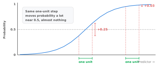
An odds ratio is the factor by which the odds of the outcome are multiplied for a one-unit increase in a predictor, holding the others constant. Exponentiate the predictor’s coefficient and you get its odds ratio.
An odds ratio of 1 means no association. Above 1 the odds increase with the predictor: 1.5 means the odds are 50% higher per unit, and 2.0 means they double. Below 1 the odds decrease: 0.5 means they halve. Because the scale is multiplicative, 2.0 and 0.5 are equal and opposite effects. On the printed scale 0.5 looks only half as far from 1 as 2.0 does, so compare effects in opposite directions with care.
Two practical points. For a continuous predictor, “per unit” means per unit as measured. An odds ratio per milligram is not directly comparable with one per ten milligrams, and reporting the unit is not optional. And the confidence interval matters more than the point estimate. An odds ratio of 3.4 with an interval from 1.05 to 11.0 is evidence of some association. The data are compatible with anything from a 5% rise in the odds to an elevenfold one. An interval that includes 1 means the data are compatible with no association at all.
One feature of those intervals surprises people. The interval on an odds ratio is not symmetric about the point estimate — 3.4 sits much closer to 1.05 than to 11.0. The asymmetry arises because the interval is computed on the log-odds scale, where it is symmetric about the coefficient, and then exponentiated along with it. Exponentiating stretches the upper half and compresses the lower half. So an odds ratio reported with a symmetric interval has almost certainly been computed the wrong way.
Reading an odds ratio as a risk ratio is a common mistake. An odds ratio compares odds. A risk ratio compares probabilities. The two are close when the outcome is rare, and they diverge sharply when it is common.
Take a baseline probability of 0.5 (odds of 1) and an odds ratio of 3. The new odds are 3, which is a probability of 0.75. The risk has gone up by a factor of 1.5, while the odds ratio reads 3. Describing that as “three times as likely” overstates the effect twofold.
Report an odds ratio as an odds ratio. If the audience needs risk, convert to predicted probabilities at stated values of the predictors. Predicted probabilities are clearer and more useful for a decision. A 2 × 2 table from a cohort or cross-sectional study gives both measures directly, without a model (see chi-square, Fisher exact or McNemar). In a case-control study only the odds ratio is valid.
There is no F-test and no ordinary R² here. The whole model, and each term in it, is tested with either a likelihood-ratio χ² test or a Wald χ² test. The likelihood-ratio test compares the fit of the model with and without the term, and is generally the more reliable of the two. The Wald test can behave badly with small samples or large effects.
Forwards, the model returns a predicted probability for any combination of predictor values. Predicted probability is the form most people want. If you then need a yes/no classification, you have to choose a probability threshold. Choosing it is a separate decision with its own trade-off between false positives and false negatives, exactly the problem ROC curves exist to display. The predicted probabilities can serve as the test score in a ROC analysis.
Backwards, inverse prediction answers the question the other way round. At what value of the predictor does the probability reach some stated level, with a confidence interval on that value? Inverse prediction is not a niche facility. The same machinery sits behind a detection limit defined as the concentration detected 95% of the time. Estimating that limit is the subject of probit analysis for the limit of detection, where probit rather than logit is the conventional link but the idea is identical.
Two failure modes are worth recognising. Separation happens when a predictor, or a combination of predictors, perfectly divides the outcomes: every case above some value is positive and every case below is negative. The likelihood has no maximum, coefficients run off towards infinity and standard errors become enormous. Separation means the predictor is extremely good; the model simply cannot express how good.
Too few events is easy to miss. It is the number of observations in the smaller outcome group that limits how many predictors a logistic model can support, not the total sample size. Two hundred observations with seven positives will not support a five-predictor model, however comfortable the total looks.
Download the logistic regression example workbook (.xlsx) — a binary logistic model of intensive care unit survival in 200 patients with 17 predictors. The analysis gives odds ratios with Wald 95% confidence intervals and likelihood-ratio tests for the model and each term. The workbook is ready to open in the Analyse-it trial.
The example workbook is downloading.
It opens in Excel on its own — the data and the finished results are both in it. Analyse-it is what lets you change the analysis and re-run it, try the same study on your own data, or work through it to see how the software handles it.
Every feature from all five editions for 15 days.
Reporting an odds ratio as “times more likely”. That phrase describes a risk ratio, and for a common outcome the two differ substantially.
Quoting an odds ratio without its interval or its unit. Both are needed before the number means anything.
Fitting a linear regression to a 0/1 response. It can predict impossible probabilities and violates the assumptions from the outset.
Counting the total sample rather than the events. The smaller outcome group is what limits how complex a model you can support.
Treating a 0.5 probability threshold as given. It is a choice, and rarely the right one when the two kinds of error carry different costs.
Ignoring wildly large coefficients and standard errors. That is usually separation, not a spectacular finding.
Analyse-it fits binary logistic regression in Fit Model, inside Excel:
Every feature from all five editions for 15 days. Logistic regression is part of the Standard edition, so it is in every Analyse-it edition, from US$ 155 a year. Validated against NIST Standard Reference Datasets.