
Simple regression relates one response to one predictor. Multiple regression relates it to several at once, and that is a genuine change in kind rather than in scale. Each coefficient is no longer “the effect of this predictor” but “the effect of this predictor holding the others constant”: an adjusted effect. Read the coefficients as unadjusted effects and you will misinterpret nearly every model you fit.
Take a coefficient of 2.4 on a predictor. Among observations that agree on every other predictor in the model, a one-unit increase in that predictor is associated with a 2.4-unit increase in the response. Change the other predictors in the model and this number can change too, in size and sometimes in sign.
The change is not a defect but the mechanism by which regression adjusts for confounding. Adjustment is most of the reason to fit a multiple model in the first place. But a coefficient has no meaning independent of the model it sits in. Quoting one without saying what else was in the model tells you very little.
Two further numbers help. A confidence interval on each coefficient shows how well the data pin it down, and is often the more informative number. A coefficient of 2.4 with an interval from 0.1 to 4.7 is a weak finding presented as a precise one. Standardised betas express each coefficient in standard deviations rather than original units, which lets you compare the relative contribution of predictors measured on entirely different scales.
When two predictors are strongly correlated with each other, the model cannot tell their effects apart. The fit still succeeds, with no error message, but the coefficients become unstable. You may see large standard errors, wide intervals, and signs that flip when you add or drop another correlated predictor. Watch in particular for individually non-significant terms in a model that is highly significant overall, which is the classic signature.
The variance inflation factor (VIF) quantifies collinearity, one value per predictor. The VIF measures how much each coefficient’s variance is inflated by that predictor’s correlation with the others. VIFs near 1 are fine, and values above about 5 deserve a look. Above 10, collinearity is serious and the coefficients concerned cannot be interpreted separately with any confidence.
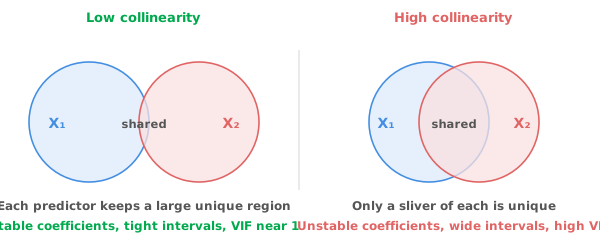
What to do about it depends on your purpose. If you are predicting, collinearity is largely harmless: predictions stay good even when individual coefficients are unstable, provided new observations show the same correlation between the predictors. If you are interpreting coefficients, collinearity is fatal. The practical options are to drop one of the pair, combine them into a single index, or collect data that breaks the correlation.
R² never decreases when you add a predictor. Add enough noise variables and it will approach 1 while the model becomes worthless outside the data it was fitted on. R² cannot compare models with different numbers of terms.
Adjusted R² penalises each additional term and can decrease, which makes it usable for that comparison. AIC and BIC do the same job more formally, trading fit against complexity. Lower is better, and only differences between models fitted to the same data are meaningful. BIC penalises extra terms more heavily than AIC, so it tends to select smaller models. BIC is therefore a reasonable default when the aim is explanation rather than raw predictive accuracy.
Whichever you use, resist automatic selection. Stepwise procedures that add and drop terms by p-value run a large number of implicit tests. The model that emerges has confidence intervals and p-values that are no longer valid, because they take no account of the search that produced them. Subject knowledge about which predictors belong in the model is worth more than any search over the ones that happen to be in the spreadsheet.
Multiple regression is not restricted to continuous predictors. A categorical variable enters through coded indicator terms. Under dummy (reference) coding its coefficients are differences from a reference level. Under effect coding, which Analyse-it uses for nominal factors, they are differences from the average across levels. Combined with continuous predictors, the model is then an ANCOVA. Add an interaction between a categorical and a continuous predictor and you are asking whether the slope differs between groups, which is often the most interesting question available.
Curvature is handled the same way, by adding polynomial terms. The model stays linear in its parameters no matter how bent the fitted curve looks. A logarithmic, exponential or power fit describes a genuinely non-linear relationship, such as growth that slows as the predictor increases or exponential decay, better than a high-order polynomial. A high-order polynomial will follow noise at the edges of the data and misbehave badly just outside them.
One warning applies to every kind of term: continuous, categorical or polynomial. A model with many terms fitted to a modest number of observations will describe that dataset beautifully and generalise poorly. Each term costs a degree of freedom, and there are only so many to spend.
With correlated predictors, part of the explained variation could be credited to more than one term. How you split it is what the sums-of-squares types decide. Type I (sequential) tests each term against what is left after the preceding terms, so it depends on the order they enter. Type III (partial) tests each term against everything else in the model, so it does not. Type III answers “is this term earning its place, given the rest?”, which is usually the question you want. The same distinction is set out for factors in one-way, two-way and multi-factor ANOVA.
None of the above tells you the model is the right shape. Curvature, non-constant variance and influential observations are all invisible in a coefficient table. A leverage plot isolates one term’s contribution after accounting for everything else. The plot is the cleanest way to see whether a particular predictor is really earning its coefficient or being propped up by two observations. Reading residual diagnostics covers the full set.
Download the multiple regression example workbook (.xlsx) — pulse rate against three continuous and five categorical predictors, ready to open in the Analyse-it trial. The workbook gives parameter estimates with confidence intervals and VIFs, F tests for each term, leverage plots, residual diagnostics and the outlier and influence plot.
The example workbook is downloading.
It opens in Excel on its own — the data and the finished results are both in it. Analyse-it is what lets you change the analysis and re-run it, try the same study on your own data, or work through it to see how the software handles it.
Every feature from all five editions for 15 days.
Reading a coefficient as an unadjusted effect. It is the effect with the other predictors held constant, and it changes when they change.
Comparing models on R². It cannot decrease. Use adjusted R², AIC or BIC instead, and prefer a model you can justify.
Interpreting coefficients with high VIFs. The model cannot separate predictors that carry the same information, however confident the output looks.
Trusting p-values from a stepwise search. They ignore all the models that were tried and discarded on the way.
Extrapolating beyond the data. A fitted model describes the range it was fitted over. Polynomials in particular go wrong quickly outside it.
Concluding causation from an adjusted coefficient. Adjusting for the confounders you measured is not the same as adjusting for the ones you did not.
Analyse-it fits the model in Fit Model, inside Excel:
Every feature from all five editions for 15 days. Regression is part of the Standard edition, so it is in every Analyse-it edition, from US$ 155 a year. Validated against NIST Standard Reference Datasets. See logistic regression for a yes/no response.