
Analysis of variance has an unhelpful name: it compares means, and it does so by partitioning variance. If several groups really have the same mean, their means will differ only as much as the variation within the groups leads you to expect. When the group means differ by substantially more than that, they are not all the same.
The F statistic is the ratio of the between-group and within-group mean squares. If every group shares one mean, both estimate the same noise variance and F is close to 1. The p-value is how often a ratio at least that large would arise by chance under that hypothesis.
One-way ANOVA is the direct extension of the two-sample t-test: one factor (supplier, dose, operator, batch) at three or more levels, and one continuous response. One-way ANOVA assumes the observations are independent, the residuals are approximately normal and the groups have similar variance.
Two alternatives exist if the last two assumptions do not hold. If the variances differ markedly, Welch’s ANOVA relaxes the equal-variance assumption the same way Welch’s t-test does, and it is the safer default whenever group sizes are unequal. If normality is in real doubt, not just unproven, the Kruskal-Wallis test compares the groups through ranks instead. Levene’s and Brown-Forsythe tests check the variance assumption directly, and so does Bartlett’s, though it is itself sensitive to non-normality.
The result is a single F-test, which, if significant, says only that the means are not all equal. The F-test does not say which ones differ. The temptation to follow it with a string of t-tests is exactly the trap multiple comparison procedures exist to avoid.
Real experiments rarely vary just one thing. You might have three primers and two application methods, four suppliers and two shifts, a treatment and a baseline covariate. Fitting a separate one-way ANOVA for each factor is not the same analysis, and it is usually worse. Each one ignores the variation the other factor explains, inflating the residual and making both effects harder to see.
A multi-factor model puts them in together. Each factor gets a test that accounts for the others, the residual shrinks down to what neither factor explains, and you can ask whether the factors interact.
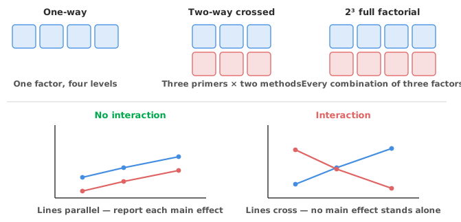
An interaction means the effect of one factor depends on the level of another. Primer A might outperform primer B when dipped and underperform it when sprayed. Both main effects could look modest or absent while the interaction is large, because averaging over the other factor cancels the two opposite effects out.
Interactions are the main reason to fit a multi-factor model, and they come with a reporting rule that is easy to miss. When an interaction is present, do not interpret the main effects on their own. “Primer A is better” is not true if it is only better when dipped. Report the effect at each level of the other factor, and let the interaction plot carry the finding. Two lines that cross say more than any table could.
A related structure shows up in method validation. In a precision study, runs are nested within days, and the goal is not to test those factors but to estimate how much variation each contributes. Those contributions are the precision components, estimated by a variance-component analysis of the nested design rather than an F-test. The same machinery underpins robustness testing with factorial designs, where the point of the design is to vary several factors at once.
Sometimes something continuous and measurable influences the response without being what you are testing: baseline severity, ambient temperature, sample age. Adding it to the model as a covariate turns the analysis into ANCOVA. The covariate absorbs variation that would otherwise sit in the residual. The factor you care about is then tested against a smaller residual, and the group means are reported adjusted to a common covariate value.
Adjusted means are what you should quote from an ANCOVA. Raw group means still carry whatever imbalance in the covariate the groups happened to have. The adjustment assumes the covariate has the same slope in every group, so test the factor × covariate interaction before relying on it.
In a multi-factor model with unequal cell counts, the factors overlap: some variation could be credited to either one. How you split it is what the sums-of-squares types settle. Type I (sequential) gives each term only the variation left after the terms entered before it, so the answer depends on the order you list them in. Type III (partial) gives each term the variation it uniquely explains after every other term, so it does not depend on order.
For a balanced factorial design with no covariates, where every cell has the same count, the two agree and the distinction never comes up. For an unbalanced design they can differ, sometimes substantially. Type III is the sensible default for asking “does this factor matter, given everything else in the model?”, which is nearly always the question you actually want answered. Type I is the right tool when the terms have a genuine hierarchy and you want to test them in a deliberate sequence. Adding a quadratic term after the linear one is the standard case.
An ANOVA table summarises a fitted model, and it is only as trustworthy as that model is. The same diagnostics that apply to regression apply here too, because underneath it is the same machinery. Residual plots expose non-constant variance and curvature. A residual distribution plot and a normal Q-Q plot address the normality assumption. An outlier and influence plot, studentised residuals against leverage with each point sized by Cook’s D, shows whether a handful of observations are driving the whole result. Reading residual diagnostics covers what each pattern means.
Download the two-way ANOVA example workbook (.xlsx): aircraft primer paint adhesion across three primers and two application methods, with F-tests for each term, adjusted effect means, main effect plots and Tukey-Kramer comparisons on both factors. The 2³ full factorial example adds all two-way and three-way interactions, and the ANCOVA example shows a three-level factor adjusted for a continuous covariate.
The example workbook is downloading.
It opens in Excel on its own — the data and the finished results are both in it. Analyse-it is what lets you change the analysis and re-run it, try the same study on your own data, or work through it to see how the software handles it.
Every feature from all five editions for 15 days.
Reporting main effects in the presence of an interaction. If the effect of one factor depends on another, its average effect describes no single condition. Report it at each level instead.
Running separate one-way ANOVAs instead of one multi-factor model. You lose the interaction entirely and inflate the residual in both analyses.
Following a significant F with unadjusted t-tests. Six groups give fifteen pairwise comparisons; at 5% each, the chance of a false positive somewhere is over a third.
Quoting raw means from an ANCOVA. The point of the covariate is adjustment. Report the adjusted effect means.
Assuming Type I and Type III agree. In an unbalanced design they need not, and reporting whichever the software defaulted to is not really a decision.
Treating repeated measurements as independent. Several measurements on the same subject belong in a within-subjects design, not stacked up as separate observations.
Analyse-it fits the model your design calls for, inside Excel:
Every feature from all five editions for 15 days. ANOVA and ANCOVA are part of the Standard edition, so they are in every Analyse-it edition, from US$ 155 a year. Validated against NIST Standard Reference Datasets. Read on for choosing a multiple comparison procedure.